Understanding Simple Linear Regression Models

A simple linear regression model is one of the most fundamental tools in econometrics. It helps us understand that labor economists have documented a persistent relationship between years of schooling and hourly earnings across developed and developing nations. Simple linear regression quantifies this relationship by fitting a straight line through observed data points. The method isolates the effect of a single explanatory variable on an outcome, forming the baseline for advanced econometric modeling. Analyzing data from the National Bureau of Economic Research reveals how wages shift systematically with education.

Understanding this baseline model allows analysts to interpret slope coefficients, assess goodness of fit, and recognize the boundaries of bivariate estimation. The technique traces its origins to Sir Francis Galton, who observed that tall parents tended to have children shorter than themselves, leading to a “regression” toward the average height. This biological observation evolved into a foundational mathematical tool for empirical economics, allowing researchers to separate systematic trends from random noise.

The Ordinary Least Squares Criterion

Econometrics bridges economic theory and observed data. Theory proposes that education enhances productivity, which translates into higher wages. Data provides scattered observations of individuals with different schooling levels earning different wages. The scatter plot does not align perfectly along a straight edge. Simple linear regression provides a mechanism to draw the line that best summarizes this cloud of points.

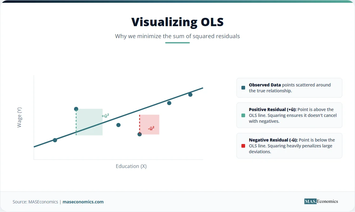
The “best fit” criterion relies on minimizing the sum of squared residuals. A residual measures the vertical distance between an observed data point and the fitted line. Some points sit above the line, yielding positive residuals. Others fall below, yielding negative residuals. Squaring these distances accomplishes two things. Squaring makes all values positive, preventing positive and negative distances from canceling out. Squaring also penalizes larger distances more heavily than smaller ones, ensuring the line does not ignore extreme outliers.

Alternative fitting criteria exist. Minimizing the sum of absolute deviations creates a line robust to outliers, but the absolute value function lacks a continuous derivative at zero, complicating mathematical optimization. Minimizing the maximum residual creates a minimax fit, which heavily prioritizes the single worst-fitting point. The resulting technique, Ordinary Least Squares (OLS), dominates empirical economics because of its computational simplicity and its optimal properties under specific conditions. The foundations of econometrics rest on this minimization principle.

The geometry of OLS reveals an important property. The OLS regression line always passes through the point of sample means, \( (\bar{X}, \bar{Y}) \). This point acts as the fulcrum of a seesaw. The line balances the positive and negative moments around this center of gravity. Understanding this balancing act clarifies why extreme outliers can disproportionately tilt the line, pulling the estimated slope toward their position. The method treats all squared deviations equally, meaning an observation far from the mean exerts a large quadratic pull on the estimated parameters.

Derivation of the OLS Estimators

The population regression function defines the true, unobserved relationship between the dependent variable \( Y \) and the independent variable \( X \). It includes an intercept \( \beta_0 \), a slope \( \beta_1 \), and an error term \( u_i \) representing unobserved factors.

Since the population parameters remain unknown, analysts estimate them using sample data. The sample regression function uses the estimated intercept \( \hat{\beta}_0 \) and the estimated slope \( \hat{\beta}_1 \).

The residual \( \hat{u}_i \) represents the difference between the observed value and the fitted value.

OLS minimizes the Sum of Squared Residuals (SSR). The objective function is:

To find the minimum, calculus dictates setting the partial derivatives with respect to \( \hat{\beta}_0 \) and \( \hat{\beta}_1 \) equal to zero.

Dividing by -2 and expanding the summations yields the system of normal equations. The first normal equation establishes that the regression line passes through the sample means of X and Y. Specifically, \( \bar{Y} = \hat{\beta}_0 + \hat{\beta}_1 \bar{X} \). Solving for the intercept gives:

The second normal equation provides the formula for the slope. Substituting the expression for the intercept into the second equation and rearranging terms produces the standard OLS slope estimator.

The slope estimator equals the sample covariance between X and Y divided by the sample variance of X. This mathematical relationship confirms that the slope captures how Y covaries with X relative to how X varies with itself. When mastering multiple regression models, this covariance mechanism expands into matrix algebra, but the core intuition remains identical.

Under the Gauss-Markov assumptions, OLS achieves the Best Linear Unbiased Estimator (BLUE) property. Unbiasedness means the expected value of the estimator equals the true population parameter. Efficiency means the variance of the OLS estimator is smaller than the variance of any other linear unbiased estimator. These properties explain why OLS serves as the workhorse of empirical economics, provided its strict assumptions hold in the data.

Interpreting OLS Output

Consider a dataset tracking the hourly wages of 198 workers and their years of formal education. Applying the OLS formulas yields an intercept of 4.50 and a slope of 1.20. The estimated equation becomes:

The intercept of 4.50 indicates the predicted hourly wage for a worker with zero years of education. While this literal interpretation lacks practical relevance because almost everyone has some schooling, the intercept anchors the line at the correct vertical position. The slope of 1.20 means that each additional year of education is associated with a $1.20 increase in hourly wages. Over a standard four-year degree, this translates to a predicted hourly wage increase of $4.80, reflecting a meaningful economic return.

Standard errors measure the precision of these estimates. They quantify the average distance that the sample estimates fall from the true population parameters. A t-statistic results from dividing the coefficient by its standard error. Large t-statistics indicate that the estimated effect is large relative to the sampling variation. P-values translate t-statistics into probabilities. A p-value below 0.01 means there is less than a 1% probability of observing such a large slope if the true population slope were actually zero.

Table 1 reports the full OLS output. The coefficient on education carries three significance stars, denoting a p-value below 0.01. The R-squared value of 0.340 indicates that years of education explain 34% of the variation in hourly wages. The remaining 66% stems from unobserved factors like experience, ability, and local labor market conditions, which belong in the error term.

Table 1. OLS Estimation: Hourly Wages on Years of Education

Variable	Coefficient	Std. Error	t-statistic	p-value
Intercept	4.50***	(0.85)	5.29	<0.001
Education (years)	1.20***	(0.12)	10.00	<0.001
R-squared	0.340
Adj. R-squared	0.338
F-statistic	100.0 (p < 0.001)
Observations	198

Note: ^* p<0.10, ^** p<0.05, ^*** p<0.01. Standard errors in parentheses. Stylized canonical example.

The scatter plot visualizes this relationship. The teal points represent the individual observations of wages and education. The upward-sloping line represents the OLS fit. The shaded mint region around the line represents the 95% confidence interval for the predicted values. Notice how the confidence interval narrows near the mean of the education variable and widens at the extremes, reflecting greater certainty where data is concentrated. This funnel shape emerges because the estimation error compounds as predictions move further from the center of the data.

Applications of Simple Linear Regression

Empirical economics relies on bivariate estimation to establish baseline relationships before adding control variables. Labor economics consistently documents the return to education. A National Bureau of Economic Research working paper details how instrumental variables confirm the causal impact of schooling on earnings, building directly on the simple OLS framework. The World Bank education sector uses similar models to assess how school attainment links to national income across developing nations. In these applications, the OLS slope provides a first approximation of economic returns, guiding policy decisions on public investment in education.

Macroeconomic forecasting also depends on linear relationships. The IMF World Economic Outlook often models the connection between GDP growth and unemployment, known as Okun’s Law. Analysts regress the change in unemployment on GDP growth. The slope captures how many jobs an economy creates per percentage point of growth. When the slope changes over time, structural shifts in labor markets become apparent. A flatter Okun’s Law coefficient suggests that economic growth generates fewer jobs than it historically did, prompting central banks to adjust monetary policy frameworks. Time series econometrics requires careful handling of autocorrelation when estimating these macro relationships over long horizons.

Policy evaluation uses simple regression to measure the initial impact of interventions. Researchers at the OECD Economics Department evaluate the link between fiscal stimulus percentages and GDP growth rates across member states. The estimated coefficient provides a raw multiplier before controlling for institutional differences. Similarly, the Bank for International Settlements publishes analysis on the relationship between credit growth and financial stability, often starting with bivariate scatter plots to identify systemic risk buildups. Central banks, including the Federal Reserve, use simple regression to inspect the Phillips curve relationship between inflation and unemployment. In financial economics, the Capital Asset Pricing Model relies on a simple regression of individual stock returns on market returns, where the estimated slope represents the stock’s systematic risk, or beta.

Limitations and Assumption Violations

Bivariate estimation provides a clean summary of data, but it imposes strict assumptions that often fail in practice. The OLS estimator remains unbiased only if the error term is uncorrelated with the independent variable. Omitted variable bias occurs when an unobserved factor influences both the dependent and independent variables. In the wage equation, innate ability affects both education and wages. Because ability sits in the error term, the OLS slope on education captures both the true return to schooling and the return to innate ability, inflating the estimate.

The mathematical formula for omitted variable bias clarifies the direction and magnitude of the error. Let the true model include education and ability, but the estimated model omits ability. The expected value of the estimated slope on education equals the true slope plus the product of two terms. The first term is the coefficient of the omitted variable in the true model. The second term is the coefficient from a regression of the omitted variable on the included variable. If ability positively affects wages and positively correlates with education, the bias is positive. The bivariate estimate overstates the true return to education. Instrumental variables offer a solution by finding a variable that shifts education but has no direct link to ability.

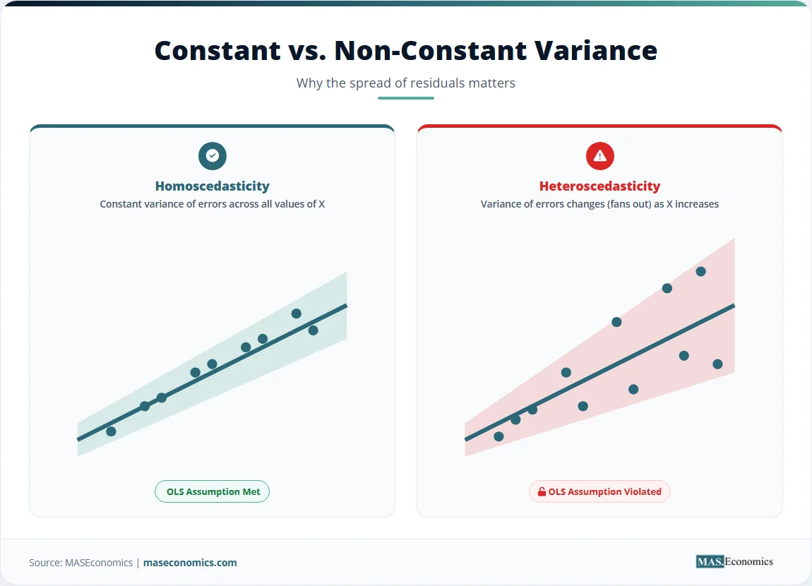
Homoscedasticity requires the variance of the errors to remain constant across all values of the independent variable. Wage data typically violates this assumption. The variance of wages for college graduates exceeds the variance for high school dropouts because higher education opens access to a wider range of occupations, from modestly paid teaching roles to highly compensated corporate law positions. Detecting this violation requires formal heteroscedasticity tests. When errors exhibit non-constant variance, OLS remains unbiased but inefficient, and standard errors become unreliable. Robust standard errors correct the inference, though autocorrelation presents additional complications in time series data.

Linearity assumes the conditional expectation of the dependent variable is a linear function of the independent variable. Economic relationships often exhibit nonlinearities. The return to education might increase at higher levels of schooling, producing a convex pattern. A simple straight line misrepresents this curvature, leading to systematic prediction errors. Nonlinear econometric models or logarithmic transformations address this issue. Model selection criteria help determine whether adding polynomial terms improves the fit enough to justify the added complexity.

MASEconomics Explains

Conclusion

Simple linear regression provides the baseline mechanism for summarizing the relationship between two economic variables. The OLS derivation minimizes the sum of squared residuals, producing a line of best fit defined by an intercept and a slope. The slope captures the expected change in the dependent variable for a one-unit change in the independent variable. The framework offers mathematical elegance, yet its estimates rely heavily on assumptions of linearity, homoscedasticity, and exogeneity. Violations of these assumptions introduce bias and inefficiency, requiring more advanced tools like multiple regression, robust standard errors, and instrumental variables to isolate causal effects in complex economic systems.

Thank you for reading! If you found this helpful, share it with friends and spread the knowledge. Happy learning with MASEconomics