In time series econometrics, stationarity is a crucial concept that determines how a time series behaves over time. For economists and researchers working with economic data, understanding whether a time series is stationary or non-stationary directly influences how models are specified and interpreted. In this post, we will explore the concept of stationarity, why it is important, and how unit root tests like the Dickey-Fuller test help detect non-stationary series.
What is Stationarity in Time Series?
Stationarity refers to the statistical properties of a time series—specifically, the mean, variance, and autocovariance—remaining constant over time. For a series to be stationary, it must fulfill the following conditions:
Constant Mean
The expected value (mean) of the series remains the same across time. For example, if we are analyzing monthly inflation rates, a stationary process implies that the average inflation stays consistent over several years, without a persistent upward or downward trend.
Constant Variance
The variability around the mean does not change over time. For instance, a stationary stock return series would show consistent fluctuation around its mean, regardless of economic cycles. Non-stationary data, on the other hand, might exhibit increasing volatility during financial crises, signaling changing variance.
Constant Autocovariance
The relationship between values in the series depends only on the time lag, not the specific time point. For example, the correlation between today’s and yesterday’s stock prices should be the same as that between last month’s and the previous month’s prices if the series is stationary.
In contrast, non-stationary series often show trends, changing variance, or evolving patterns over time. Many macroeconomic variables, such as GDP, inflation, and stock prices, are non-stationary because they tend to exhibit growth trends and cycles.

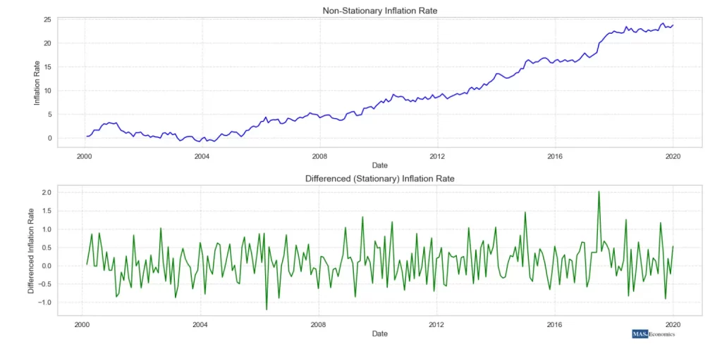
The graph above illustrates the concept of stationarity in time series analysis using synthetic inflation data. The top plot shows a non-stationary inflation rate that exhibits an upward trend over time, indicating that the mean and variance change, which can cause long-term shocks to persist. The bottom plot displays the differenced inflation rate, which is stationary, meaning that the time series has a consistent mean over time, and any shocks are temporary. This comparison helps in understanding the importance of stationarity in econometric modeling and time series analysis.
Why is Stationarity Important?
The importance of stationarity lies in its implications for model stability and inference. Many econometric models, especially those in time series analysis, such as Autoregressive Moving Average (ARMA) models, rely on the assumption that the data are stationary. Here’s why this assumption is critical:
Predictability
Stationary data allows for more accurate forecasting because the underlying statistical properties remain constant over time. If a time series is non-stationary, past values may not be useful for predicting future values because the patterns could change unpredictably.
Spurious Regressions
Regressions involving non-stationary time series can lead to misleading results, known as spurious regressions. For example, two unrelated series like the price of milk and the stock market index might appear to have a strong relationship simply because they both trend over time. This can lead to incorrect conclusions about economic relationships.
Modeling Requirements
Many standard time series models, such as ARMA, ARIMA, and Vector Autoregression (VAR), require data to be stationary. Applying these models to non-stationary data can result in poor model performance and inaccurate forecasts. Therefore, transforming non-stationary data into stationary data is often a necessary step before proceeding with the analysis.
Understanding the role of stationarity ensures that time series models are stable and that inferences drawn from them are valid. Without addressing stationarity, predictions may be unreliable, leading to poor decisions based on flawed analysis.
Unit Root Tests
To determine whether a series is stationary or non-stationary, unit root tests are employed. A time series that contains a unit root is considered non-stationary, while a stationary series does not have a unit root. The most commonly used unit root tests are the Dickey-Fuller (DF) test and its augmented version, the Augmented Dickey-Fuller (ADF) test.
The Dickey-Fuller Test
The Dickey-Fuller test estimates a simple autoregressive model to check for the presence of a unit root:
Description:
- \( Y_t \) is the value of the series at time \( t \),
- \( \rho \) is a coefficient, and
- \( \epsilon_t \) is a random error term.
The test checks the null hypothesis that \( \rho = 1 \), meaning the series has a unit root and is non-stationary. The model can be rearranged as:
Description:
- \( \Delta Y_t \) is the first difference of the series, and
- \( \delta = \rho – 1 \).
If \( \delta = 0 \), the series is non-stationary. If \( \delta < 0 \), the series is stationary.
The Augmented Dickey-Fuller (ADF) Test
The ADF test expands on the Dickey-Fuller test by allowing for higher-order autoregressive processes. It includes additional lagged differences of the series to account for more complex autocorrelation structures:
The ADF test checks whether \( \gamma = 0 \). If so, the series has a unit root and is non-stationary. The inclusion of lagged differences makes the ADF test more robust when dealing with time series data that exhibit autocorrelation.
How to Apply the Dickey-Fuller Test
Let’s go through the steps of applying the Dickey-Fuller test to determine whether an economic time series, such as inflation rates, is stationary.
- Visual Inspection: Start by plotting the time series. If the series exhibits a clear trend or changing volatility, it is likely non-stationary.
- Differencing the Data: Apply the first difference to the data if it appears non-stationary. This involves subtracting each value of the series from its previous value:
Differencing can help transform a non-stationary series into a stationary one, making it suitable for analysis.
- Performing the Test: Conduct the Dickey-Fuller or ADF test on both the original and differenced data using statistical software like R, Python, or EViews.
- Interpreting the Results: The test results provide a test statistic and a critical value. If the test statistic is less than the critical value, the null hypothesis of a unit root is rejected, indicating that the series is stationary.
Testing for Stationarity in Inflation Rates
Let’s consider an example of testing for stationarity in inflation rates. Suppose we have monthly inflation data and want to determine whether inflation follows a stationary process.
- Visualize the Data: First, plot the inflation data. A visible trend might suggest non-stationarity.
- Perform the ADF Test: Use Python’s
statsmodelslibrary to perform the ADF test on the data.
- Interpret the Output: If the ADF test confirms a unit root, the series is non-stationary, meaning that shocks to inflation could have long-lasting effects. If the test rejects the null hypothesis, inflation is stationary, indicating that any shocks have only temporary effects.
Stationarity and Differencing
If a series is non-stationary, differencing is a common solution. For example, taking the first difference of a non-stationary inflation series can help remove trends and transform it into a stationary series. This is crucial when applying models like ARMA or ARIMA, which assume stationarity for accurate forecasting.
Conclusion
Stationarity is a cornerstone of time series econometrics, influencing how models are built, interpreted, and applied in practice. Understanding whether a time series is stationary determines the stability and reliability of predictions made using models like ARMA or VAR. Ignoring non-stationarity can lead to spurious relationships, misleading forecasts, and poor decision-making, especially in fields like finance and macroeconomic policy.
Through unit root tests like the Dickey-Fuller and Augmented Dickey-Fuller tests, analysts can detect non-stationarity and take corrective actions, such as differencing or transforming the data. This process ensures that the insights drawn from econometric models are statistically valid and meaningful in a real-world context.
FAQs:
What is stationarity in time series econometrics?
Stationarity in time series refers to a condition where the statistical properties of a series—such as mean, variance, and autocovariance—remain constant over time. A stationary time series does not exhibit trends or changing volatility, making it predictable and suitable for certain econometric models like ARMA and ARIMA.
Why is stationarity important in time series analysis?
Stationarity is crucial because it ensures the stability of time series models, allowing for reliable forecasting. Without stationarity, models may produce spurious regressions and inaccurate predictions, leading to misleading interpretations and poor decision-making in economic analysis.
What is the difference between stationary and non-stationary time series?
A stationary time series has a constant mean, variance, and autocovariance over time, meaning it does not exhibit trends or seasonal patterns. Non-stationary time series, on the other hand, display trends, changing variance, or evolving patterns, making them less predictable and requiring transformation (like differencing) for accurate modeling.
How can you test for stationarity in a time series?
To test for stationarity, analysts often use unit root tests like the Dickey-Fuller (DF) or Augmented Dickey-Fuller (ADF) tests. These tests assess whether a time series has a unit root, which indicates non-stationarity. If the test rejects the null hypothesis of a unit root, the series is considered stationary.
What is the role of the Dickey-Fuller test in time series econometrics?
The Dickey-Fuller test is used to determine whether a time series is stationary or has a unit root, indicating non-stationarity. It checks if the series’ differences are stationary, helping analysts decide whether to use differencing or other transformations before applying time series models like ARMA.
How do you make a non-stationary series stationary?
To make a non-stationary series stationary, one common method is differencing, where each value in the series is subtracted from its previous value. This process can remove trends or seasonality, making the series suitable for time series modeling and forecasting.
Thanks for reading! If you found this helpful, share it with friends and spread the knowledge.
Happy learning with MASEconomics


