Economic relationships often unfold over time, with policies, shocks, or decisions showing delayed effects on economic variables. For instance, an increase in oil prices may impact GDP gradually over several quarters. To capture these delayed responses, econometricians use distributed lag models.
These models analyze how the effects of an independent variable, such as oil prices or government spending, influence a dependent variable like GDP or inflation over time. By incorporating lag structures, distributed lag models reveal the dynamic behavior of economic systems, making them essential tools for empirical economic analysis.
Why Lag Structures Matter in Economic Analysis
Lag structures are vital for accurately analyzing time-dependent relationships. Economic variables do not always reLag structures play a central role in understanding how economic variables respond to shocks or policies over time. Unlike instantaneous relationships, most economic interactions involve delays due to the complexity of decision-making processes and adjustment mechanisms. Failing to account for these delays can lead to misleading conclusions, as significant effects may be overlooked or misattributed.
The Nature of Lag Effects
Adjustment Delays
Firms and households rarely adjust their behavior immediately when faced with economic changes. For instance, businesses may take several quarters to react to changes in interest rates due to the time required for budgeting, planning, and implementing new strategies.
Habit Formation
Consumers’ decisions are often influenced by habits or past experiences. For example, changes in income may not immediately translate into higher consumption as individuals adjust their spending gradually over time.
Expectations and Anticipation
Economic agents may anticipate policy changes, leading to staggered responses. For instance, a government’s announcement of future infrastructure spending may influence current investment decisions, creating a lagged response in GDP growth.
Illustrating the Lagged Effects of Shocks
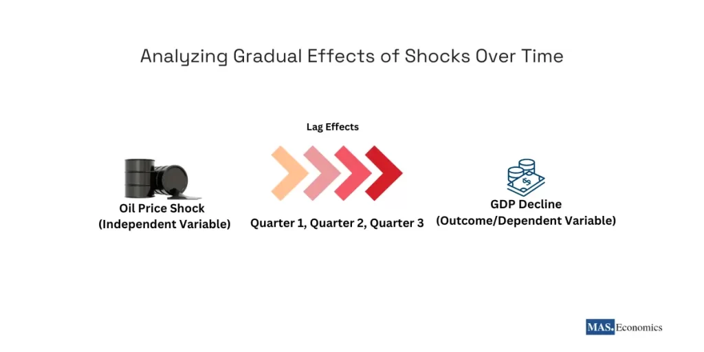
To better understand how shocks propagate through the economy over time, consider the example of an oil price shock. When oil prices rise, the impact on GDP is not immediate but occurs gradually as businesses and consumers adjust to higher production and transportation costs. The effects may unfold over successive quarters, leading to a lagged decline in economic output.
The illustration below visually demonstrates this concept:

As shown in the image, the lag effects spread over Quarter 1, Quarter 2, and Quarter 3, capturing the gradual transmission of the shock. By explicitly modeling these delays, distributed lag models allow economists to measure both the timing and magnitude of these effects, providing a clearer picture of how economic shocks influence key variables over time.
Importance of Explicit Lag Structures
By explicitly incorporating lag structures into econometric models, researchers can uncover the timing and magnitude of relationships between variables. Distributed lag models help answer important questions such as:
- How long does it take for a monetary policy change to impact inflation?
- When will fiscal spending start influencing economic output?
- What is the cumulative effect of oil price shocks on GDP over multiple quarters?
Incorporating lags allows economists to map the transmission of shocks over time, improving the accuracy of policy evaluation, forecasting, and economic analysis.
Understanding Finite Lag Models (Almon Lag)
Finite lag models are a type of distributed lag model where the effects of an independent variable persist for a fixed number of time periods. These models are particularly useful when we believe the influence of an explanatory variable eventually disappears after a certain lag length.
For example, an increase in government spending today may continue to impact economic output for a year or two, but after that, the effect is expected to diminish entirely.
Mathematically, a finite lag model can be represented as:
Here:
The coefficients
The Challenge of Multicollinearity
While finite lag models are straightforward to understand, a major challenge arises during estimation: multicollinearity. Multicollinearity occurs because the lagged values of
To address this issue, econometricians use the Almon Lag Model, which imposes a structure on the lag coefficients to simplify estimation.
The Almon Lag Model
The Almon lag model assumes that the lag coefficients follow a smooth polynomial function. Instead of estimating each coefficient separately, the Almon model expresses the lag coefficients as:
Where:
By assuming that the lag coefficients follow a smooth curve, the Almon lag model reduces the number of parameters to estimate. This helps mitigate multicollinearity and ensures that the estimated lag structure is both smooth and interpretable.
Example: Government Spending and Economic Output
Suppose we are analyzing the effect of government spending on GDP growth over four quarters. In a standard finite lag model, we would estimate four separate coefficients:
In the Almon lag model, we impose a quadratic polynomial structure on the lag coefficients:
This approach assumes that the effects of government spending are smooth and follow a predictable pattern over the four quarters, making the results easier to interpret. The Almon lag model simplifies the estimation process while retaining the dynamic relationship between government spending and GDP growth.
Infinite Lag Models Explained (Koyck Model)
While finite lag models assume that the effect of an independent variable disappears after a certain time, infinite lag models allow the effects to persist indefinitely. These models are particularly useful for analyzing relationships where shocks or changes have long-term, decaying effects.
For example, changes in interest rates may influence inflation for many years, but the impact gradually diminishes over time.
The Koyck Model: Simplifying Infinite Lags
The most commonly used infinite lag model is the Koyck Model, which introduces a geometric decay structure. This model assumes that the effects of an independent variable decline gradually and proportionally over time.
The Koyck model can be written as:
Here:
The key idea behind the Koyck model is that the cumulative effect of past values of
How the Decay Parameter Works
The parameter
- If
- If
Example: Interest Rates and Inflation
Suppose we analyze the impact of interest rate changes (
The Koyck model captures this dynamic relationship:
Here:
If
Key Differences Between Finite and Infinite Lag Models
The table below highlights the primary distinctions between finite lag models (e.g., the Almon lag) and infinite lag models (e.g., the Koyck model):
| Aspect | Finite Lag Models | Infinite Lag Models |
|---|---|---|
| Lag Length | Effects persist for a fixed number of periods. | Effects persist indefinitely but decay over time. |
| Decay | No decay is imposed on lagged effects. | Geometric decay is imposed (e.g., Koyck). |
| Model Complexity | Estimates separate coefficients for each lag. | Uses fewer parameters (includes |
| Example Model | Almon Lag Model | Koyck Model |
| Practical Use | Best for short-lived effects with a known lag structure. | Ideal for long-term effects that diminish gradually. |
| Application | Government spending and short-term GDP effects. | Interest rates and long-term inflation dynamics. |

|
||
Both finite and infinite lag models are essential tools in econometrics for analyzing time-dependent relationships between variables. Finite models, like the Almon lag, are appropriate when effects are short-lived and limited to specific time periods. On the other hand, infinite lag models, like the Koyck model, are more suitable when the effects are persistent but gradually fade over time.
Practical Applications in Economic Analysis
Lag models have critical implications for understanding real-world economic phenomena and making informed decisions. They provide a framework for analyzing dynamic relationships that unfold over time and guide policymakers, researchers, and analysts in evaluating long-term effects.
Analyzing Policy Effects
Economic policies, such as fiscal stimulus or monetary interventions, often exhibit delayed impacts. Distributed lag models allow economists to measure both the immediate effect and the cumulative long-term effect of these policies. For example:
- Fiscal Spending: The Almon lag model can determine how government spending affects output across different time periods, providing clarity on whether the majority of the impact occurs in the short term or is spread out over multiple quarters.
- Monetary Policy: The Koyck model helps estimate how interest rate adjustments influence inflation, capturing the gradual decay of monetary shocks.
Understanding Shock Transmission
Lag models are essential for evaluating how unexpected shocks propagate through the economy. For instance:
- Oil Price Shocks: A sudden rise in oil prices may cause production costs to increase, influencing GDP growth over several quarters.
- Exchange Rate Fluctuations: Changes in currency values may affect trade balances with lags, as importers and exporters adjust to new price levels.
Forecasting Economic Trends
By analyzing lagged relationships, econometricians can make better forecasts about economic trends. For example, historical relationships between consumer spending and income levels can help predict future consumption patterns, accounting for adjustment delays and habit persistence.
Key Implication
The use of lag models goes beyond academic research—they are vital tools for businesses, governments, and central banks to evaluate the timing and efficacy of economic decisions. By modeling lags accurately, decision-makers can better anticipate outcomes and design more effective strategies.
Conclusion
Distributed lag models are essential in econometrics for analyzing how economic shocks, policies, or decisions influence outcomes over time. By accounting for delayed responses, these models provide a clearer view of dynamic relationships that static analyses often miss.
Finite lag models, such as the Almon lag, are effective when the effects of an independent variable are short-lived, offering a simplified estimation by assuming a polynomial structure. Infinite lag models, like the Koyck model, capture long-term impacts with a geometric decay structure, efficiently addressing persistent effects without requiring an infinite number of coefficients.
These models enhance the precision of economic analysis, enabling better forecasting and evaluation of policy impacts while providing valuable insights into the dynamic nature of economic systems.
FAQs:
What are distributed lag models?
Distributed lag models capture how the effects of an independent variable, such as policy changes or economic shocks, influence a dependent variable over time. They incorporate lag structures to reveal the delayed responses of economic variables.
Why are lag structures important in economic analysis?
Lag structures account for delays in how economic agents respond to changes. For example, firms or households may take time to adjust their behavior after an interest rate change. Ignoring these delays can result in misleading conclusions about the timing and magnitude of relationships.
What is the difference between finite and infinite lag models?
Finite lag models assume that the effects of an independent variable persist for a limited number of periods before disappearing. Infinite lag models allow effects to persist indefinitely but assume they decay gradually over time, often using structures like the Koyck model.
What is the Almon lag model?
The Almon lag model is a finite lag model that uses a polynomial structure to smooth the lag coefficients. This helps mitigate multicollinearity issues that arise when lagged values of an independent variable are highly correlated.
How does the Koyck model handle infinite lags?
The Koyck model introduces a geometric decay structure, where the effect of an independent variable diminishes gradually over time. By including the lagged dependent variable, the model efficiently captures long-term relationships without estimating an infinite number of coefficients.
What are the practical applications of distributed lag models?
Distributed lag models are used to analyze policy impacts, shock transmission, and forecasting trends. For instance, they help measure how fiscal spending influences GDP over time or how interest rate changes affect inflation dynamics.
Thanks for reading! Share this with friends and spread the knowledge if you found it helpful.
Happy learning with MASEconomics


