Advanced Difference-in-Differences Methods: Beyond Two-Way Fixed Effects

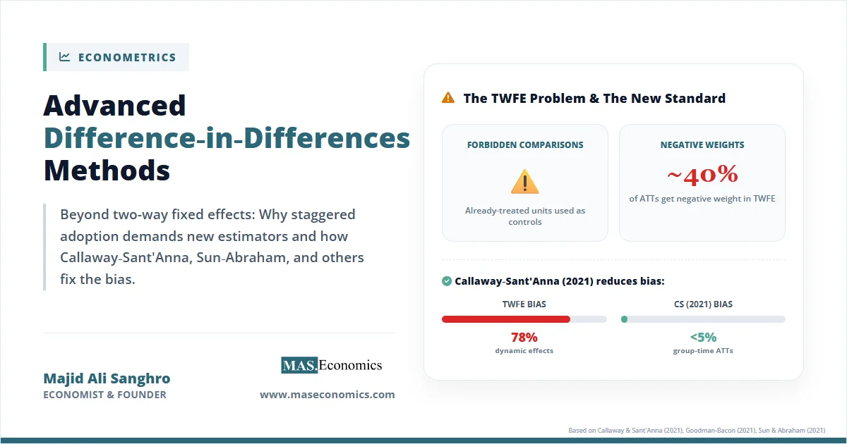
Between 2018 and 2024, a quiet revolution swept through applied econometrics. A series of papers by Callaway and Sant’Anna (2021), Goodman-Bacon (2021), Sun and Abraham (2021), Borusyak, Jaravel, and Spiess (2024), and de Chaisemartin and D’Haultfoeuille (2020) demonstrated that the workhorse method used in thousands of published policy evaluations, two-way fixed effects (TWFE) regression with staggered treatment adoption, can produce severely biased estimates when treatment effects are heterogeneous across time or across groups. Simulation studies found that TWFE bias reached 66 to 79% in settings with dynamic treatment effects, turning statistically significant results into artefacts of the estimation procedure rather than evidence of policy impact. The advanced difference-in-differences methods developed in response have fundamentally changed how empirical economists estimate causal effects, and any researcher still running a standard TWFE regression on staggered policy data without robustness checks is using a method the profession has effectively discredited.

The stakes are not merely academic. Difference-in-differences (DiD) is the most widely used quasi-experimental design in economics, political science, public health, and education research. Minimum wage studies, healthcare policy evaluations, environmental regulation assessments, and labour market analyses all rely on DiD. When the method produces biased results, the policy conclusions drawn from those results are wrong. The new estimators correct these biases by decomposing the staggered design into a series of “clean” two-by-two comparisons, each grounded in transparent assumptions about parallel trends and treatment effect heterogeneity.

The Canonical DiD

In its simplest form, difference-in-differences compares the change in outcomes over time between a treated group and a control group. With two periods (before and after treatment) and two groups (treated and untreated), the DiD estimator is:

The first difference removes time-invariant unobserved heterogeneity (fixed differences between the groups). The second difference removes common time trends (shocks that affect both groups equally). What remains, under the parallel trends assumption, is the causal effect of the treatment.

The identifying assumption, parallel trends, states that in the absence of treatment, the average outcome for the treated group would have evolved in parallel with the average outcome for the control group. This assumption cannot be tested directly (since we cannot observe the counterfactual), but researchers typically examine pre-treatment trends for evidence of divergence.

In the two-period, two-group case, the DiD estimator is straightforward, well-understood, and uncontroversial. The problems arise when researchers extend this framework to settings with multiple time periods and staggered treatment adoption, which is what the vast majority of real-world policy evaluations require.

The TWFE Problem

The standard econometric implementation of DiD in staggered settings is the two-way fixed effects regression:

where \( \alpha_i \) are unit fixed effects, \( \lambda_t \) are time fixed effects, \( D_{it} \) is a treatment indicator, and \( \delta \) is the parameter of interest. For decades, applied economists treated \( \delta \) as the average treatment effect on the treated (ATT). This interpretation is correct when treatment effects are homogeneous: the same for all units and constant over time. When treatment effects vary across groups or evolve dynamically, the TWFE estimator can produce estimates that are severely biased, including estimates with the wrong sign.

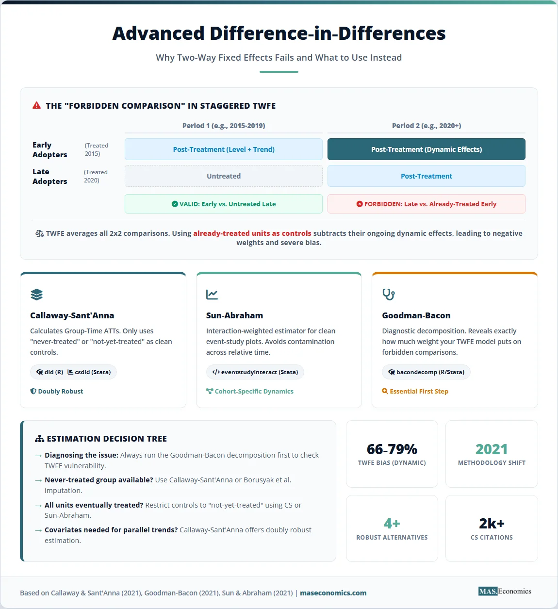
Andrew Goodman-Bacon’s 2021 Journal of Econometrics paper provided the definitive diagnosis. He proved that the TWFE estimator is a weighted average of all possible two-by-two DiD comparisons that can be constructed from the data, but the weights are not all positive. Some comparisons receive negative weight, and some use already-treated units as controls for later-treated units (the “forbidden comparisons”).

The mechanism is intuitive. When a state adopts a policy in 2015, and another adopts the same policy in 2020, the TWFE regression implicitly uses the 2015 state as a control for the 2020 state during the 2015 to 2020 period. But the 2015 state is already treated during this period. If the treatment effect is growing over time (dynamic effects), the 2015 state’s outcome is being pushed up by the treatment, making it a bad comparison for the 2020 state’s pre-treatment trend. The resulting estimate can be biased downward, upward, or even flip sign.

Goodman-Bacon’s decomposition theorem shows exactly how much weight each two-by-two comparison receives in the TWFE estimate, allowing researchers to diagnose the severity of the problem in their specific application. In simulations with dynamic treatment effects, TWFE bias ranged from 66 to 79%, rendering the estimates essentially meaningless.

Problem	Description	When It Occurs	Severity
Forbidden comparisons	Already-treated units used as controls for later-treated units	Always in staggered designs without never-treated group	Can flip sign of estimate
Negative weights	Some group-time treatment effects receive negative weight in TWFE	When treatment effects are heterogeneous across groups	Bias of 30-80%
Dynamic effect contamination	Event-study coefficients contaminated by effects at other horizons	When treatment effects evolve over time post-treatment	Bias of 66-79% in simulations
Pre-trend masking	Forbidden comparisons can mask or create false pre-trends	In standard event-study specifications with staggered timing	Misleading inference

The Callaway-Sant’Anna Estimator

Brantly Callaway and Pedro Sant’Anna’s 2021 Journal of Econometrics paper has become the most widely adopted solution, with over 2,000 citations and a dedicated R package (did) and Stata implementation. Their approach is built on a simple but powerful idea: define the causal parameter of interest at the most disaggregated level possible, then aggregate transparently.

Step 1: Group-Time Average Treatment Effects

The fundamental building block is the group-time average treatment effect, \( ATT(g, t) \): the average effect of treatment on units in group \( g \) (those first treated at time \( g \)) at time \( t \). For each combination of treatment cohort and calendar time, the estimator constructs a clean two-by-two DiD comparison using only not-yet-treated (or never-treated) units as controls:

This comparison is “clean” because it never uses already-treated units as controls. Each \( ATT(g, t) \) relies on a transparent parallel trends assumption: in the absence of treatment, the average outcome for group \( g \) would have evolved in parallel with the average outcome for the not-yet-treated comparison group between period \( g – 1 \) and period \( t \).

Step 2: Flexible Aggregation

Once all group-time ATTs are estimated, Callaway and Sant’Anna propose multiple aggregation schemes depending on the research question:

Event-study aggregation: Average across groups for each event time (time since treatment) to produce a standard event-study plot showing how the treatment effect evolves post-treatment:

Group-specific aggregation: Average across time for each group to show which cohorts experienced larger or smaller effects:

Overall aggregation: A single summary measure of the average treatment effect:

The transparency of this approach is its strength. Every aggregation step is explicit, every weight is known, and the researcher can inspect heterogeneity across groups and across event time before deciding how to summarise the results.

Step 3: Covariates and Doubly Robust Estimation

In many applications, parallel trends hold only conditional on observed covariates (conditional parallel trends). Callaway and Sant’Anna accommodate this through three estimation strategies: outcome regression, inverse probability weighting, and a doubly robust estimator that combines both. The doubly robust estimator is consistent if either the outcome regression model or the propensity score model is correctly specified, providing an extra layer of protection against misspecification.

Alternative Estimators

Sun and Abraham (2021): Interaction-Weighted Estimator

Sun and Abraham take a regression-based approach. Instead of running a single TWFE regression, they interact treatment indicators with cohort indicators, estimating separate effects for each cohort at each event time. Their “interaction-weighted” estimator constructs a weighted average of these cohort-specific effects, with weights proportional to cohort size. This approach is particularly useful for researchers comfortable with regression frameworks who want to produce clean event-study plots without the negative-weight contamination of standard TWFE event studies.

Borusyak, Jaravel, and Spiess (2024): Imputation Estimator

The imputation approach (also independently proposed by Gardner, 2021) uses a two-stage procedure. In the first stage, the researcher estimates the unit and time fixed effects using only the untreated observations (observations where \( D_{it} = 0 \)). In the second stage, these estimated fixed effects are used to impute the counterfactual outcomes for treated observations. The treatment effect is the difference between the observed and imputed outcomes. This approach imposes a stronger parallel trends assumption (parallel trends in all pre-treatment periods, not just the last one) but can be more efficient when this assumption holds.

Wooldridge (2021): Extended TWFE

Jeffrey Wooldridge, author of the most widely used graduate econometrics textbook, proposed a modified TWFE regression that includes interactions between treatment indicators and group/time indicators. His approach nests the other estimators as special cases under certain conditions and has the advantage of being implementable within the familiar OLS regression framework. Wooldridge shows that under standard error component assumptions, the extended TWFE estimator can be both best linear unbiased (BLUE) and asymptotically efficient.

Estimator	Key Innovation	Parallel Trends Assumption	Software
Callaway-Sant’Anna (2021)	Group-time ATTs with flexible aggregation; doubly robust	Weaker: last pre-treatment period only	did (R), csdid (Stata)
Sun-Abraham (2021)	Interaction-weighted estimator for event studies	Weaker: last pre-treatment period only	eventstudyinteract (Stata)
Borusyak-Jaravel-Spiess (2024)	Imputation of counterfactuals from untreated observations	Stronger: all pre-treatment periods	did_imputation (Stata), didimputation (R)
Wooldridge (2021)	Extended TWFE with group-time interactions; BLUE under standard assumptions	Stronger: all pre-treatment periods	jwdid (Stata)
de Chaisemartin-D’Haultfoeuille (2020)	Identifies conditions for negative weights in TWFE; robust estimator	Flexible	did_multiplegt (Stata/R)
Goodman-Bacon (2021)	Diagnostic decomposition of TWFE into component 2×2 DiDs	Diagnostic tool (not estimator)	bacondecomp (R/Stata)

Parallel Trends

The parallel trends assumption remains the identification backbone of all DiD designs, whether traditional or advanced. No estimator eliminates the need for this assumption; the new methods simply ensure that the estimator does not introduce additional bias beyond what a violation of parallel trends would produce.

Pre-trend testing is standard practice: researchers examine whether outcomes for treated and control groups evolved in parallel during the pre-treatment period. Under the Callaway-Sant’Anna framework, this is done by computing \( ATT(g, t) \) for periods \( t < g \) (before group \( g \) is treated). If these pre-treatment ATTs are statistically indistinguishable from zero, the parallel trends assumption is supported (though not proven).

Jonathan Roth’s work on sensitivity analysis for parallel trends has become increasingly influential. Roth (2022) demonstrates that pre-trends tests have low statistical power: they can fail to reject parallel trends even when the assumption is violated. He proposes a sensitivity analysis framework (implemented in the HonestDiD R package) that allows researchers to report how large a violation of parallel trends would need to be to overturn their conclusions.

Rambachan and Roth (2023) extend this framework by proposing “honest” confidence intervals that remain valid under specified violations of parallel trends. These intervals are wider than standard confidence intervals but provide reliable coverage even when the assumption is imperfect, a significant advance for applied researchers working with observational data.

From Contaminated to Clean

Event-study designs, which plot treatment effects at each time period relative to the treatment date, are the standard way to visualise DiD results. The typical event-study specification includes leads and lags of the treatment indicator:

where \( G_i \) is the time unit \( i \) is first treated and the coefficients \( \gamma_e \) trace out the treatment effect at each event time \( e \). Under homogeneous effects, this produces a clean plot showing zero effects pre-treatment (validating parallel trends) and the evolving treatment effect post-treatment.

Sun and Abraham (2021) showed that under heterogeneous treatment effects, these event-study coefficients are contaminated by treatment effects at other horizons, producing misleading dynamic patterns. Their interaction-weighted estimator resolves this by computing separate event-study coefficients for each cohort and then averaging them with appropriate weights.

The Callaway-Sant’Anna framework produces event-study plots through aggregation of group-time ATTs by event time. This approach is transparent: each point on the event-study plot is a weighted average of identified \( ATT(g, t) \) parameters, with weights that the researcher controls and can report.

When to Use Which Method

The choice among advanced DiD estimators depends on the specific empirical context. Several considerations guide the decision:

Strength of parallel trends assumption: If the researcher believes parallel trends hold in all pre-treatment periods, the Borusyak-Jaravel-Spiess and Wooldridge estimators can be more efficient because they use all pre-treatment data for identification. If parallel trends are plausible only in the period immediately before treatment (perhaps because of pre-treatment confounders in earlier periods), the Callaway-Sant’Anna and Sun-Abraham estimators are more appropriate.

Presence of covariates: If parallel trends hold only conditional on observed covariates, the Callaway-Sant’Anna doubly robust estimator is particularly well-suited. Wooldridge’s approach also accommodates covariates through interaction terms in the extended TWFE regression.

Availability of never-treated units: Some estimators use never-treated units as the comparison group; others use not-yet-treated units. When a never-treated group exists and is comparable to the treated groups, it provides a cleaner comparison. When all units are eventually treated, the not-yet-treated approach must be used.

Computational requirements: Wooldridge’s extended TWFE is the simplest to implement (it is a regression). The Callaway-Sant’Anna estimator requires the did package and uses bootstrap inference. The Borusyak-Jaravel-Spiess imputation estimator is computationally efficient and produces analytic standard errors.

Regardless of which estimator is chosen, running the Goodman-Bacon diagnostic is always recommended. It reveals the composition of the TWFE estimate and identifies whether forbidden comparisons or negative weights are substantial in the specific dataset.

How the New Methods Change Conclusions

Several influential policy evaluations have been revisited using the new DiD methods, with substantive changes in conclusions.

Minimum wage effects: Callaway and Sant’Anna re-estimated the effect of minimum wage increases on teen employment using their new framework and found qualitatively different results from standard TWFE. The group-time ATTs revealed significant heterogeneity across states and over time that the TWFE coefficient had masked.

Medicaid expansion: Studies of the Affordable Care Act’s Medicaid expansion have been revisited using staggered DiD methods. The staggered rollout across US states (some expanding in 2014, others later, some never) is precisely the setting where TWFE can produce biased estimates. The Callaway-Sant’Anna and Sun-Abraham estimators produced estimates that were qualitatively similar to TWFE for this application but with wider confidence intervals, reflecting the reduced precision that comes from avoiding forbidden comparisons.

Environmental regulation: Studies of environmental policies (cap-and-trade programmes, emissions regulations) with staggered state-level adoption have been particularly affected. The dynamic treatment effects in these settings (environmental benefits accumulate over time as firms invest in cleaner technology) are precisely the conditions under which TWFE bias is most severe.

The chart makes the case for advanced DiD methods in a single visual. Under homogeneous treatment effects (the leftmost pair of bars), TWFE and Callaway-Sant’Anna produce nearly identical, unbiased estimates. The difference emerges when effects are heterogeneous or dynamic: TWFE bias escalates to 66 to 79% under dynamic treatment effects (the three rightmost scenarios), while the Callaway-Sant’Anna estimator remains well below 5% bias across all scenarios. The red bars represent the cost of using the old method; the teal bars represent the solution.

Extensions and Frontiers

The DiD revolution continues to expand into new territories. Callaway, Goodman-Bacon, and Sant’Anna (2024) extend the framework to continuous treatments (where the treatment is a dose rather than a binary indicator), showing that TWFE regressions with continuous treatment variables face analogous problems with negative weights and forbidden comparisons. De Chaisemartin and D’Haultfoeuille have extended their methods to fuzzy DiD designs (where treatment is not perfectly determined by the policy assignment) and to settings with time-varying covariates.

The connection between DiD methods and causal inference more broadly is also deepening. Synthetic control methods (Abadie, Diamond, and Hainmueller 2010), which construct comparison groups from weighted combinations of untreated units, are increasingly being combined with DiD estimators. The resulting “synthetic DiD” estimator (Arkhangelsky et al. 2021) blends the strengths of both approaches: the transparency of DiD’s parallel trends assumption with the flexibility of synthetic control’s data-driven weighting.

Machine learning methods are also entering the DiD toolkit. Doubly robust estimators can use machine learning for the nuisance parameters (outcome regressions and propensity scores), improving flexibility without sacrificing the causal interpretation. The integration of machine learning into causal inference is one of the most active frontiers in modern econometrics.

MASEconomics Explains

Conclusion

Advanced difference-in-differences methods have transformed applied econometrics. The demonstration that standard TWFE regressions can produce bias of 66 to 79% under dynamic treatment effects, a setting that describes the vast majority of real-world policy evaluations, represents one of the most consequential methodological findings in recent economics. The Callaway-Sant’Anna estimator, with its transparent group-time ATTs, flexible aggregation, and doubly robust option, has emerged as the new standard for staggered DiD designs. The Sun-Abraham interaction-weighted estimator provides a clean solution for event studies. The Borusyak-Jaravel-Spiess imputation estimator offers computational efficiency. Wooldridge’s extended TWFE maintains the familiar regression framework while correcting the bias.

The practical implication is clear: any empirical study using DiD with staggered treatment adoption should, at a minimum, run the Goodman-Bacon diagnostic to assess the severity of forbidden comparisons and negative weights, and report results from at least one heterogeneity-robust estimator alongside the standard TWFE specification. Journals, referees, and policy agencies are increasingly requiring this as a condition for publication. The methodological revolution is complete; what remains is ensuring that the applied practice catches up.

Did you find this article helpful? Share it with someone who loves economics. And remember, at MASEconomics, we make complex ideas simple.