Bond duration and convexity are the two mathematical tools that fixed-income markets use to measure how much a bond’s price moves when interest rates change. When the Federal Reserve cut rates by 50 basis points in September 2024, a 30-year US Treasury bond gained roughly 9% in price within days. A 2-year note moved less than 1%. The difference was not luck or sentiment. It was duration, and the residual gap between the linear estimate and the actual price change was convexity. Together, they form the analytical backbone of bond portfolio management, pension fund liability matching, and central bank balance sheet analysis.
The framework was built in pieces over four decades. Frederick Macaulay introduced duration in 1938 as the weighted average time to receive a bond’s cash flows. Frederick Redington formalised the idea of immunisation in 1952. Lawrence Fisher and Roman Weil extended duration to portfolio applications in 1971. Convexity, the second-order correction, became standard in trading desks during the 1980s when interest-rate volatility forced practitioners to confront the limits of linear approximation. By the time Silicon Valley Bank collapsed in March 2023, every chief risk officer in the world was using duration and convexity, though clearly not all of them well.
What Duration and Convexity Do
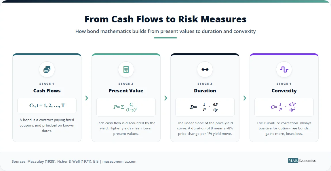
A bond is a contract that pays fixed cash flows on fixed dates. Its market price is the present value of those cash flows discounted at the prevailing yield. When the yield rises, the present value falls. When the yield falls, the present value rises. The relationship is non-linear because each cash flow is discounted by a power of the yield, and powers are not linear functions.
Duration answers the first-order question: by how much does the bond’s price change when the yield changes by a small amount? It is the slope of the price-yield curve at the current yield, scaled to give a percentage price change per unit of yield change. A bond with a duration of 8 years will fall roughly 8% in price if yields rise by 100 basis points, and rise roughly 8% if yields fall by 100 basis points.
The “roughly” matters. Because the price-yield relationship is curved, duration alone overstates the loss when yields rise and understates the gain when yields fall. Convexity is the second-order correction that captures this curvature. A bond with high convexity outperforms a bond with low convexity at the same duration, because it loses less when yields rise and gains more when yields fall. This asymmetric payoff is why convexity is valuable, and why traders pay for it.
The framework solved a practical problem that had vexed fixed-income managers since the 1930s. Two bonds with the same maturity could behave very differently. A 30-year zero-coupon bond and a 30-year bond with a 10% coupon both mature on the same date, but their interest-rate sensitivities are not the same. Macaulay’s insight was that maturity is a poor measure of risk; the timing of cash flows matters. A bond that pays most of its value early is less sensitive to rate changes than one that pays most of its value at the end. Duration captures this by computing the weighted average time of cash flows, with the weights being the present values.
Mathematical Formulation of Duration and Convexity
Consider a bond with cash flows \( C_t \) paid at times \( t = 1, 2, \ldots, T \), priced at yield \( y \). The bond’s price is the sum of discounted cash flows:
Macaulay duration, \( D_{\text{Mac}} \), is defined as the weighted average time to receive cash flows, where each weight is the share of the bond’s price contributed by that cash flow:
The weights sum to one, so Macaulay duration is measured in years. For a zero-coupon bond, all the weight sits on the maturity date, and Macaulay duration equals maturity. For a coupon bond, duration is always less than maturity, because some cash flows arrive before the final payment.
Modified duration, \( D_{\text{mod}} \), converts Macaulay duration into a price-sensitivity measure by dividing by \( (1 + y) \):
Modified duration is the negative of the percentage price change per unit change in yield, evaluated at the current yield:
This is the practical workhorse. If a bond has \( D_{\text{mod}} = 7.5 \) and yields rise by 25 basis points (0.0025), the linear estimate of the price change is:
The bond is expected to fall by about 1.88%. The estimate is good for small changes but breaks down when yield moves are large, because the price-yield curve bends.
Convexity, \( C \), is the second derivative of price with respect to yield, normalised by price:
The convexity-adjusted price change combines the linear duration term with the quadratic convexity term:
The quadratic term is always positive for standard bonds, because \( (\Delta y)^2 \) is always positive and convexity is positive for option-free fixed-income securities. This is the source of the asymmetry. When yields rise, duration predicts a large loss, but convexity adds back a partial recovery. When yields fall, duration predicts a large gain, and convexity adds even more on top.
The derivation comes directly from a Taylor expansion of the price function around the current yield \( y_0 \):
Dividing through by \( P(y_0) \) and substituting the definitions yields the standard duration-convexity approximation. Higher-order terms exist but are negligible for yield changes under 200 basis points on standard bonds.
The variables, their definitions, and typical ranges are summarised below.
| Symbol | Definition | Units | Typical Range (Investment-Grade) |
|---|---|---|---|
| \( P \) | Bond price (present value of cash flows) | Currency | $95–$110 per $100 face |
| \( C_t \) | Cash flow at time \( t \) (coupon and/or principal) | Currency | $2–$5 (semi-annual coupon) |
| \( y \) | Yield to maturity | Decimal | 0.02–0.07 |
| \( T \) | Maturity | Years | 2–30 |
| \( D_{\text{Mac}} \) | Macaulay duration (weighted average time of cash flows) | Years | 1.9–17 |
| \( D_{\text{mod}} \) | Modified duration (price sensitivity) | % per 1% yield change | 1.8–16 |
| \( C \) | Convexity | Years² | 4–300 |
| \( \Delta y \) | Yield change | Decimal | ±0.005 (typical daily move) |
For a callable bond, the formulas need adjustment. The issuer’s right to redeem early caps the upside when yields fall, producing what practitioners call negative convexity. Mortgage-backed securities exhibit this property because homeowners refinance when rates drop. The standard formula gives effective duration and effective convexity by computing price changes numerically at small upward and downward yield shocks rather than analytically.
Assumptions and Limitations of the Framework
The duration-convexity framework rests on three assumptions that are convenient but unrealistic. First, the yield curve is assumed to shift in parallel. A 25-basis-point change in the 2-year yield is assumed to move the 10-year and 30-year yields by exactly 25 basis points as well. In practice, yield curves twist and bend. The 2024 Federal Reserve easing cycle saw the 2-year yield fall by more than 100 basis points while the 30-year yield rose modestly, a steepening that no parallel-shift model would have predicted.
Second, cash flows are assumed to be fixed and known. This holds for non-callable government bonds and high-grade corporates, but fails for any security with embedded optionality. Mortgage-backed securities, callable corporates, putable bonds, convertible bonds, and floating-rate notes all have cash flows that depend on the path of interest rates. For these instruments, the effective duration computed from a stochastic model replaces the closed-form expression. The Bank for International Settlements has documented how mortgage convexity hedging by US agencies amplifies bond market moves during periods of rapid rate change.
Third, the framework treats yield as the single driver of price. Credit spreads, liquidity premia, and term premia are absorbed into the yield itself, but they move independently. A bond’s price can fall even when Treasury yields are stable if the issuer’s credit deteriorates. Duration measures only the interest-rate component of risk, not the spread component. A separate measure called spread duration is needed for the latter.
The Taylor approximation also breaks down at large yield changes. For moves above 200 basis points, third-order terms become non-trivial. Practitioners add a third-order correction or revert to full revaluation, computing the bond price at the new yield directly.
Two further limits matter for portfolio managers. Duration is additive in dollar terms but not in yield terms across bonds with different yields. The portfolio duration is a value-weighted average of individual durations only when all bonds have the same yield. When yields differ, the aggregation requires care. And duration changes as yields change. A bond’s duration today is not its duration after a 100-basis-point move, because the new duration reflects the new discount factors. This is why convexity hedges need rebalancing.
Empirical Evidence for Duration and Convexity
The duration-convexity framework has been tested extensively in academic and practitioner literature, and the results are consistent. For small yield changes on standard bonds, the linear duration approximation captures more than 95% of the actual price change. For changes between 50 and 200 basis points, adding the convexity term raises the explanatory power to above 99%.
The 2022–2023 monetary tightening cycle was the largest stress test of the framework in two decades. Between March 2022 and July 2023, the Federal Reserve raised the federal funds rate from a range of 0.00%–0.25% to 5.25%–5.50%, the steepest tightening since 1981. The Bloomberg US Aggregate Bond Index, which has a duration of roughly 6 years, fell by roughly 13% in 2022, the worst year on record. The duration framework predicted the direction and approximate magnitude of the loss; the actual outcome was within 1 percentage point of the duration-implied estimate after accounting for spread changes, according to IMF Global Financial Stability Report analysis.
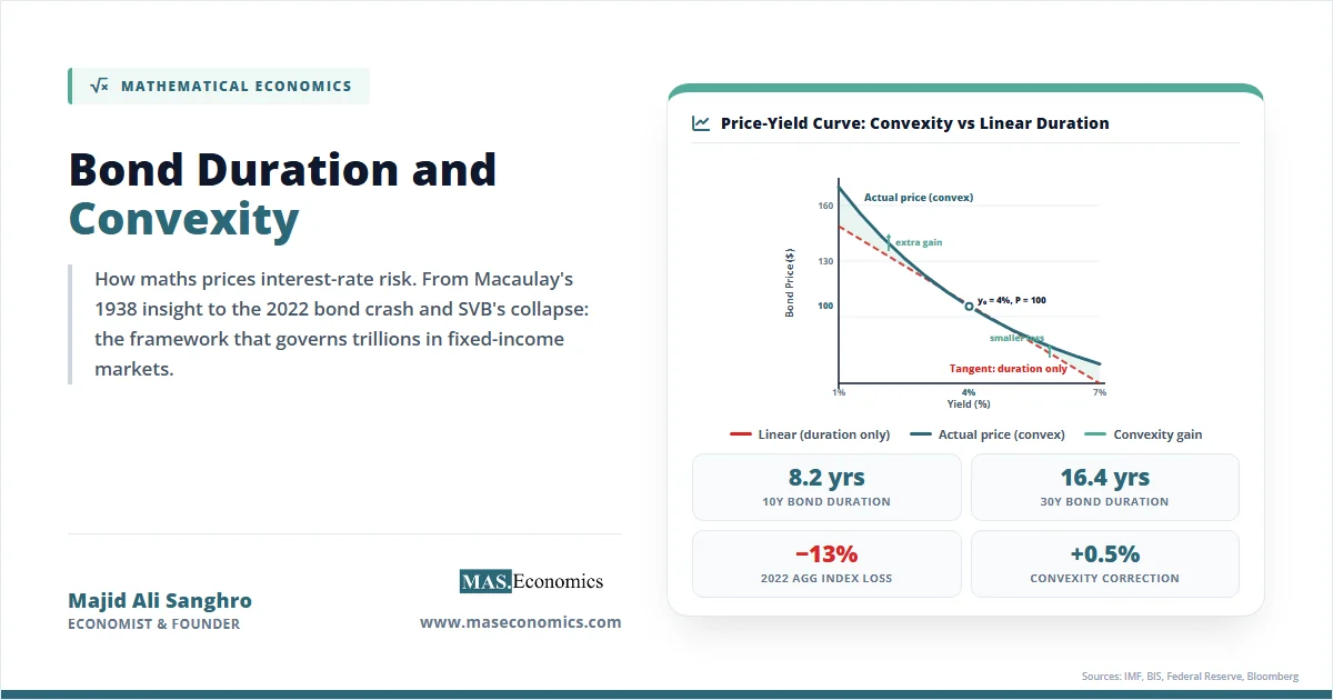
The chart below illustrates the framework’s central prediction: how duration and convexity together approximate price changes for bonds of different maturities under a parallel yield shock.
Chart: Estimated price change for option-free US Treasury bonds under a parallel yield shift from a starting yield of 4.0%. Duration-only estimate compared with duration-plus-convexity estimate and full revaluation. Calculations based on standard semi-annual coupon conventions.
The chart shows three findings that recur across empirical work. First, the duration-only line diverges from the actual price change as yield moves grow. Second, the convexity correction closes most of that gap, with residual error under 0.3 percentage points even at 200-basis-point shocks. Third, longer-duration bonds have higher convexity in absolute terms, which is why the gap between duration-only and full revaluation widens dramatically for the 30-year bond.
Studies on portfolio immunisation, where duration-matched portfolios are constructed to fund known liabilities, find that simple Macaulay duration matching reduces interest-rate risk by 80%–90% over horizons of one to three years. The remaining risk comes from non-parallel yield curve shifts, which require multi-factor extensions such as key-rate durations or principal-component analysis. Federal Reserve research has documented how pension funds and insurance companies use duration matching to fund long-dated liabilities, with empirical results closely tracking theoretical predictions when liabilities are well-defined.
The framework’s most public failure was Silicon Valley Bank in March 2023. SVB held a portfolio of long-duration Treasury and agency mortgage-backed securities that had been purchased at low yields during 2020 and 2021. As yields rose, the duration framework predicted exactly the unrealised losses that materialised. SVB’s $15 billion in unrealised losses at the end of 2022 was not a surprise to anyone running the numbers; it was a balance sheet consequence that any bond textbook could have predicted. The bank’s collapse was a failure of risk management, not of the mathematics. The numbers worked. Nobody acted on them in time.
The Importance of Duration and Convexity
Duration and convexity are not academic abstractions. They are the operating language of fixed-income markets, and the four largest applications shape trillions of dollars of decisions every year.
The first application is in central bank policy analysis. When the Federal Reserve, European Central Bank, or Bank of England changes interest rates, the immediate impact on the financial system runs through the duration of bond portfolios. The Bank of England’s 2022 intervention in the gilt market was triggered by a duration crisis. UK pension funds running liability-driven investment strategies had used leverage to extend the duration of their assets to match the duration of their long-dated liabilities. When 30-year gilt yields spiked by more than 100 basis points in a day, the value of those leveraged positions collapsed, generating margin calls that forced further selling. The Bank of England’s Financial Stability Report documented how the duration mismatch and the convexity exposure of these strategies amplified the move and forced the central bank to step in. The framework explained the crisis precisely. It also pointed to the cure.
The second application is in commercial bank balance sheet management. Banks fund themselves with short-duration liabilities (deposits) and invest in longer-duration assets (loans, mortgages, Treasury securities). The mismatch is the classic source of bank profitability and bank risk. The Federal Deposit Insurance Corporation requires banks to report interest-rate risk metrics that are essentially duration-based. The Basel Committee on Banking Supervision’s Interest Rate Risk in the Banking Book framework mandates a 200-basis-point parallel shock test as the standard regulatory measure, and it computes duration-based estimates of the impact on economic value. The 2023 US regional banking stress, which started with SVB and spread to First Republic and others, was at heart a duration story. Banks that had loaded up on long-duration mortgage-backed securities during the low-rate era found themselves with assets worth 15%–20% less than book value. The Federal Reserve’s review of SVB’s failure identified inadequate interest-rate risk management as a primary cause.
The third application is in pension fund and insurance company liability matching. Defined-benefit pension plans owe payments decades into the future. The present value of those liabilities behaves like a long-duration bond. When yields fall, the present value of liabilities rises, and the funded ratio falls unless assets rise by the same amount. Duration matching, also known as immunisation, structures the asset portfolio so that its duration equals the duration of the liabilities. Convexity matching adds a second-order condition that reduces residual risk. The largest US pension fund, the California Public Employees’ Retirement System (CalPERS), and the largest UK pension fund schemes use duration-based liability matching as standard practice. The Australian Prudential Regulation Authority’s prudential standards for insurance companies embed duration metrics as core regulatory capital inputs.
The fourth application is in active portfolio management. Bond portfolio managers express views on interest rates by adjusting the duration of their portfolios relative to a benchmark. A manager bullish on bonds (expecting yields to fall) extends duration above the benchmark. A bearish manager shortens duration. The decision is sharper than the directional call alone. A manager extending duration through a bond with high convexity gets asymmetric upside; the same duration extension through a callable bond may have negative convexity, capping the gain. The convexity choice matters as much as the duration choice. Hedge funds running relative-value strategies in fixed income build positions designed to harvest convexity at attractive prices, profiting when realised volatility exceeds the convexity-implied breakeven.
The framework also shapes how households experience monetary policy. When the Fed raises rates, the duration of mortgage-backed securities held by banks and the Federal Reserve itself rises (because prepayments slow when rates rise). This “extension risk” lengthens the effective duration of the system’s bond holdings exactly when bond losses are mounting, a feedback loop that amplifies the impact of tightening cycles. The opposite happens when rates fall: prepayments accelerate, mortgage-backed security duration shortens, and investors lose the duration they thought they had. This negative convexity is the reason mortgage-backed securities trade at higher yields than Treasury securities of similar duration; investors demand compensation for the option they have implicitly written to homeowners.
Duration and convexity also matter in the analysis of sovereign debt sustainability. A country that funds itself with short-duration debt is more exposed to rising rates than one that has issued long-duration bonds. The UK’s gilt market, with an average maturity above 14 years, is among the longest in the developed world; the US Treasury market, with an average maturity of around 6 years, is much shorter. When rates rise, debt-service costs rise faster in countries with shorter average duration, an effect documented in the IMF Fiscal Monitor analysis. The Australian Office of Financial Management and the Canadian Department of Finance publish duration metrics for their sovereign debt portfolios precisely because these numbers determine fiscal exposure.
For the typical investor in the United States, the United Kingdom, Canada, or Australia, duration and convexity show up indirectly. The bond fund in a 401(k), RRSP, or ISA has a duration printed on its fact sheet. That number, multiplied by the change in interest rates, is roughly how much the fund will gain or lose. A target-date retirement fund glides from longer-duration to shorter-duration bonds as the investor approaches retirement, because the duration of the implicit liability (the need for stable income) shortens as time passes. The mathematics that started with Macaulay’s 1938 paper now governs trillions of dollars in retirement savings.
MASEconomics Explains
Four economic concepts behind bond duration and convexity
Conclusion
Bond duration and convexity together provide the mathematical scaffolding for measuring interest-rate risk in fixed-income markets. Duration captures the linear sensitivity of bond prices to yield changes; convexity corrects for the curvature that duration alone misses. The framework, built from a Taylor expansion of the present-value formula, has stood up to nine decades of empirical testing and forms the basis of regulatory standards at the Federal Reserve, the European Central Bank, the Bank of England, and the Bank for International Settlements. Pension funds use it to match liabilities. Banks use it to manage balance sheet risk. Treasury debt managers use it to gauge fiscal exposure. The 2022 bond market drawdown and the 2023 banking stress were not surprises to anyone running the duration numbers. The mathematics worked. The institutions that ignored it did not.
Did you find this article helpful? Share it with someone who loves economics. And remember, at MASEconomics, we make complex ideas simple.