GARCH model: Volatility Clustering in Markets

Daily S&P 500 returns do not move with a constant error variance. Calm periods cluster together, crisis periods cluster together, and a large shock today often predicts high volatility tomorrow. A GARCH model turns that empirical pattern into an estimable conditional variance process.

The problem is not that stock returns are easy to forecast. Mean returns are often weakly predictable at daily frequency. The more persistent object is the size of the shock. Financial time series commonly show low-volatility stretches, sudden bursts, and slow decay back toward calmer conditions. A constant-variance regression treats those episodes as noise. GARCH treats them as the object of interest.

The canonical example uses daily S&P 500 returns, with the index level taken conceptually from FRED’s S&P 500 daily series. The parameters below are stylized for exposition, but the econometric logic follows Engle’s ARCH model, Bollerslev’s generalized ARCH model, and the financial-risk tradition that uses conditional volatility for Value-at-Risk, stress testing, and capital allocation.

When Volatility Clusters: The 1987 Crash and Beyond

Equity returns exhibit a recurring asymmetry between predictability in direction and predictability in risk. The sign of tomorrow’s S&P 500 return is difficult to forecast. The scale of tomorrow’s movement is often more predictable because volatility comes in clusters. A quiet week tends to be followed by quiet days. A crash week tends to be followed by wider daily swings, even when the market direction changes.

This is the statistical failure behind homoskedastic models of financial returns. In a constant-variance model, the error term has the same variance every day:

That assumption is too rigid for financial returns. During normal periods, daily S&P 500 returns may move within a narrow range. During crisis periods, the same index can produce very large positive and negative movements within days. A model that averages all periods into one variance underestimates risk in turbulence and overestimates risk in calm periods.

The 1987 crash, the 2008 global financial crisis, and the March 2020 market crash all illustrate the same empirical pattern. Volatility does not rise for one day and disappear. It remains elevated because market participants adjust leverage, liquidity, margin, and expectations across several trading sessions. This persistence is exactly what conditional volatility models were built to capture.

ARCH models introduced the idea that today’s variance depends on yesterday’s squared shock. GARCH extends that logic by allowing today’s variance to depend on both yesterday’s squared shock and yesterday’s conditional variance. The second term is the key. It lets volatility decay slowly instead of forcing all persistence to pass through a long list of squared-return lags.

This connects directly to the Augmented Dickey-Fuller test. Before modelling conditional variance, the return series must be treated as a stationary object. Equity index levels are usually persistent and non-stationary, while log returns are typically closer to stationarity. The ADF article handles the unit-root question. GARCH begins after the mean equation has been transformed into a return equation suitable for volatility modelling.

GARCH Variance Mathematics

Let \( P_t \) denote the S&P 500 index level at the daily close. The continuously compounded daily return in percent is:

The simplest mean equation is a constant-mean return model:

The key object is \( \sigma_t^2 \), the conditional variance of the return shock given past information. A GARCH(1,1) specification is:

The three variance parameters have direct interpretations. The constant \( \omega \) anchors the long-run variance. The ARCH coefficient \( \alpha \) measures how strongly volatility reacts to the most recent squared shock. The GARCH coefficient \( \beta \) measures persistence from yesterday’s conditional variance. If \( \alpha \) is high, volatility reacts sharply to new market shocks. If \( \beta \) is high, volatility fades slowly.

The parameter restrictions are:

The non-negativity restrictions keep the conditional variance positive. The persistence restriction \( \alpha + \beta < 1 \) gives a finite unconditional variance. When this condition holds, the long-run variance is:

The stylized canonical example uses:

These numbers imply volatility persistence of:

The long-run conditional variance is therefore:

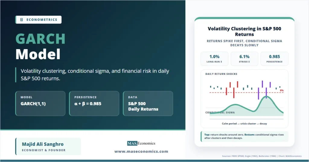
Because returns are measured in percent, the long-run daily conditional standard deviation is \( \sqrt{1.000}=1.000 \) percent. The model therefore says that the normal state of daily S&P 500 volatility is roughly 1 percent, but that large shocks can push conditional volatility far above that level for an extended period.

The null and alternative hypotheses depend on the volatility question. A basic test for no ARCH-type conditional heteroskedasticity is:

For a fitted GARCH(1,1), a common persistence question is:

Failure to reject persistence near one means volatility shocks decay very slowly. In the limiting case \( \alpha+\beta=1 \), the process resembles an integrated GARCH process, where shocks have permanent effects on the conditional variance. That specification may fit financial crises visually, but it removes mean reversion in volatility.

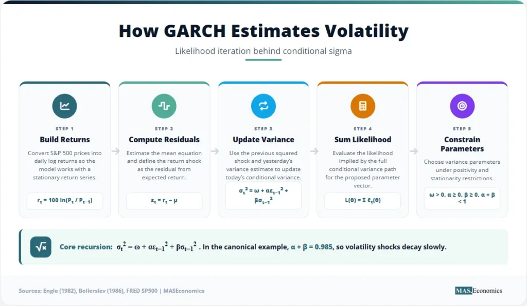
Inside the Algorithm: How GARCH Iterates

GARCH is estimated by maximum likelihood. The algorithm does not minimize squared residuals in the usual homoskedastic sense. It chooses parameters that make the observed sequence of returns most likely under the conditional variance recursion.

Let the parameter vector be:

For any candidate \( \boldsymbol{\theta} \), the algorithm first computes residuals from the mean equation:

It then initializes the first variance, often using the unconditional variance implied by the candidate parameters:

From there, the variance is computed recursively:

Assuming conditional normality, the contribution of observation \(t\) to the log-likelihood is:

The full sample log-likelihood is the sum:

The estimator is:

The iteration is mechanical. At iteration \(k\), the optimizer proposes \( \boldsymbol{\theta}^{(k)} \). The model recomputes every \( \varepsilon_t \), every \( \sigma_t^2 \), and the full log-likelihood. The optimizer then updates the candidate parameters:

where \( \mathbf{g}_k \) is the gradient of the log-likelihood, \( \mathbf{H}_k \) is a curvature approximation, and \( \lambda_k \) is a step length chosen to improve the likelihood while preserving the parameter constraints. The specific optimizer is not the economic content. The economic content is the likelihood recursion: each proposed parameter set implies a complete volatility path, and the chosen parameters are those that best fit the observed pattern of calm and turbulent returns.

This is why GARCH belongs naturally with maximum likelihood estimation. The MLE article in Phase 4 should link back to this article as a core example where likelihood is not an abstract formula. In GARCH, likelihood estimation produces the volatility series used for risk forecasts.

Reading the Output: S&P 500 Volatility

The stylized canonical example estimates a GARCH(1,1) model for daily S&P 500 log returns. The mean return is small and positive. The variance equation shows high persistence because \( \alpha+\beta=0.985 \). Standard errors appear in parentheses directly below each coefficient.

Table 1. GARCH Estimation: S&P 500 Daily Returns

Parameter	Coefficient	Std. Error	z-statistic	p-value
\( \mu \)	0.040**	(0.018)	2.22	0.026
\( \omega \)	0.015***	(0.004)	3.75	<0.001
\( \alpha \)	0.090***	(0.017)	5.29	<0.001
\( \beta \)	0.895***	(0.019)	47.11	<0.001
Persistence \( \alpha+\beta \)	0.985
Long-run variance	1.000 percent squared
Long-run sigma	1.000 percent per day
Log-likelihood	-1838.42
AIC	3684.84
BIC	3705.21
Observations	1,510 daily returns

Note: ^* p<0.10, ^** p<0.05, ^*** p<0.01. Standard errors in parentheses. Stylized canonical example based on daily S&P 500 return dynamics.

The coefficient \( \alpha=0.090 \) says new shocks matter. A large squared return yesterday raises today’s conditional variance. The coefficient \( \beta=0.895 \) says the previous variance estimate matters even more. This is the persistence channel. Once volatility rises, the model does not let it immediately fall back to the long-run average.

The sum \( \alpha+\beta=0.985 \) is close to one but below one. The process is mean-reverting, but the reversion is slow. A volatility shock has a long half-life because each day’s conditional variance carries most of yesterday’s conditional variance forward. This is why GARCH is useful for risk desks: risk does not reset at midnight.

The long-run variance calculation matches the mathematical section exactly:

The chart below shows the core GARCH pattern. Returns jump up and down around zero. Conditional sigma rises smoothly during turbulent periods and decays gradually afterward. The return series is jagged. The sigma series is persistent.

The chart gives the main interpretation. The return series has abrupt spikes. The conditional sigma line moves more smoothly because it is a filtered estimate of risk. After a large return shock, \( \varepsilon_{t-1}^2 \) raises \( \sigma_t^2 \). Then \( \beta \sigma_{t-1}^2 \) carries that elevated variance into later days. The model, therefore, separates a one-day price move from the multi-day risk environment that follows.

The decision rule is direct. The null of no conditional heteroskedasticity is rejected because \( \alpha \) and \( \beta \) are both positive and precisely estimated. The persistence condition is satisfied because \(0.985<1\), but the process is close to the boundary. In economic terms, the S&P 500 return process in this example has mean-reverting volatility, but shocks are long-lived.

When Persistence Becomes a Trap

GARCH can fail when the model’s symmetry and persistence assumptions are too restrictive. The basic GARCH(1,1) treats positive and negative shocks of the same size as having the same effect on future volatility. Equity markets often violate that symmetry. A large negative return can raise future volatility more than a large positive return of equal size. EGARCH, GJR-GARCH, and threshold GARCH models were developed to capture this leverage effect.

The second failure is fat tails. Conditional normal GARCH handles time-varying volatility, but standardized residuals may still have heavier tails than a normal distribution. A risk model that uses normal GARCH can underestimate extreme losses if the residual distribution remains too thin. Student-\(t\) innovations are often used when the standardized residuals show heavy tails.

The third failure is regime instability. The relationship between shocks and volatility can change across market structure, regulation, leverage, and liquidity regimes. A GARCH model estimated over one period may underperform when trading technology, margin rules, or macro conditions change. This problem is especially relevant when stress tests must cover events outside the estimation sample.

The fourth failure is treating a volatility forecast as a complete risk forecast. GARCH estimates conditional variance. It does not by itself determine market liquidity, jump risk, correlation breakdown, or forced selling. Those channels require additional modelling. In risk management, GARCH is one input into a broader framework, not a complete map of financial risk.

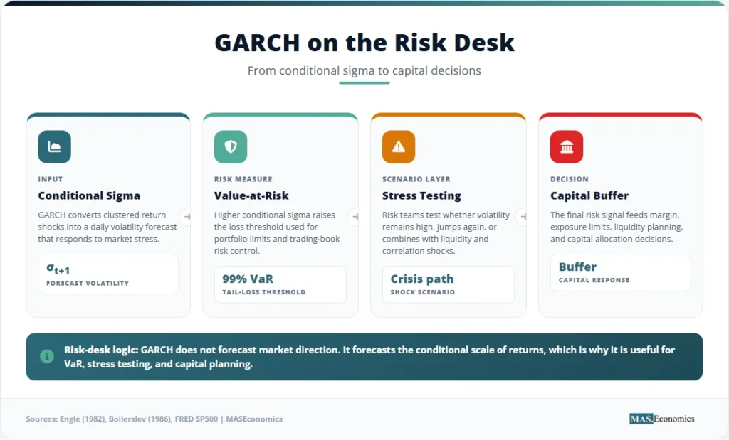
GARCH on the Risk Desk: VaR, Stress Tests, and Capital

Risk desks use conditional volatility because capital needs depend on today’s risk environment, not the average risk of the last decade. A constant historical volatility estimate can be too low after a market break and too high after a long calm period. GARCH updates the variance forecast each day using the latest squared shock and the existing volatility state.

The most common risk translation is Value-at-Risk. Under conditional normality, a one-day 99 percent VaR for a long equity position with value \(V_t\) can be written as:

The coefficient \(2.326\) is the 99 percent normal critical value. If conditional sigma rises from 1 percent to 4 percent, VaR rises sharply even if the mean return is unchanged. This is the practical role of the model: it converts a volatility cluster into a capital and limit-management signal.

Stress testing adds another layer. A desk may ask how losses change if the next shock resembles a crisis day, if volatility remains high for ten trading days, or if correlations rise while volatility rises. The BIS market-risk literature emphasizes that stress testing and VaR should be read together rather than as unrelated numbers. GARCH supplies the dynamic volatility path that can feed those calculations.

The model also helps explain why risk systems become procyclical. In calm markets, conditional sigma falls, VaR declines, and leverage constraints may loosen. After a shock, sigma rises, VaR increases, and positions may need to be cut. If many institutions respond in the same direction, the risk model can reinforce market stress. That does not make GARCH wrong. It means conditional risk estimates affect behaviour once they enter limits, margin, and capital rules.

GARCH is also connected to the broader MASEconomics econometrics library. The article on heteroscedasticity in econometric models explains why changing error variance breaks standard inference. The article on autocorrelation in time series econometrics explains why dependence in residuals matters. ARMA models and forecasting cover persistence in the mean. GARCH applies a similar time-series discipline to the variance. econometric model selection helps choose among GARCH variants using likelihood-based criteria.

The financial interpretation is therefore specific. GARCH does not forecast whether the S&P 500 will rise or fall tomorrow. It forecasts whether tomorrow’s return is likely to be drawn from a calm distribution or a turbulent distribution. That distinction is the reason the model remains a standard reference point in financial econometrics.

MASEconomics Explains

Conclusion

GARCH model estimation gives financial econometrics a disciplined way to model volatility clustering in daily returns. The S&P 500 example shows why the variance equation matters: the return itself is jagged and difficult to forecast, while conditional sigma moves in persistent clusters after market shocks. The GARCH(1,1) parameters \( \omega=0.015 \), \( \alpha=0.090 \), and \( \beta=0.895 \) imply a long-run daily sigma of 1 percent and persistence of 0.985. The model is strongest as a conditional risk tool for volatility forecasting, VaR, stress testing, and capital allocation. Its weaknesses appear when asymmetry, fat tails, regime shifts, or liquidity risk dominate the return process.

Thanks for reading! If you found this helpful, share it with friends and spread the knowledge. Happy learning with MASEconomics