Offer Curves: Reciprocal Demand and Terms of Trade

Two countries can both gain from trade, but the final trade price depends on how strongly each country wants the other country’s good. Offer curves show that reciprocal demand determines where the terms of trade settle between the limits created by comparative advantage.

The idea is central to classical and neoclassical trade theory. Comparative advantage explains why countries can gain from specialization, but it does not fully determine the international exchange ratio. Offer curves fill that gap by showing how much of one export good a country is willing to offer for different quantities of the import good.

In international trade theory, offer curves connect demand, supply, and welfare in one diagram. They show that the terms of trade are not set by production costs alone. They are also shaped by the strength and elasticity of each country’s demand for foreign goods.

Comparative advantage sets trade limits

The starting point is comparative advantage. A country exports the good it can produce at lower opportunity cost and imports the good that is relatively more expensive to produce at home. This logic explains the direction of trade.

Suppose Country A exports cloth and imports wine, while Country B exports wine and imports cloth. Trade can make both countries better off only if the international exchange ratio lies between their domestic opportunity-cost ratios. If the trade price lies outside those bounds, at least one country would prefer not to trade.

Those bounds can be written in simple terms-of-trade terms:

Mutually Beneficial Trade Range

The world relative price must lie between the two countries’ domestic opportunity-cost ratios.

Here, \(P_C/P_W\) is the relative price of cloth in terms of wine. The inequality shows the range within which trade can benefit both countries. But it does not say which exact price inside the range will prevail.

That missing price is where reciprocal demand enters. If Country A strongly wants wine and Country B weakly wants cloth, the final terms of trade may favor Country B. If Country B strongly wants cloth and Country A weakly wants wine, the final terms may favor Country A. Offer curves show this bargaining-like market outcome without treating trade as literal bargaining.

Reciprocal demand fixes the price

Reciprocal demand means each country’s demand for imports is linked to its willingness to supply exports. A country does not simply demand foreign goods. It offers its own goods in exchange. The strength of that offer depends on preferences, production possibilities, and the international relative price.

John Stuart Mill’s theory of reciprocal demand extended the Ricardian idea of comparative costs by asking how the international exchange ratio is determined within the mutually beneficial range. The key insight is that the country with stronger demand for imports tends to accept less favorable terms of trade.

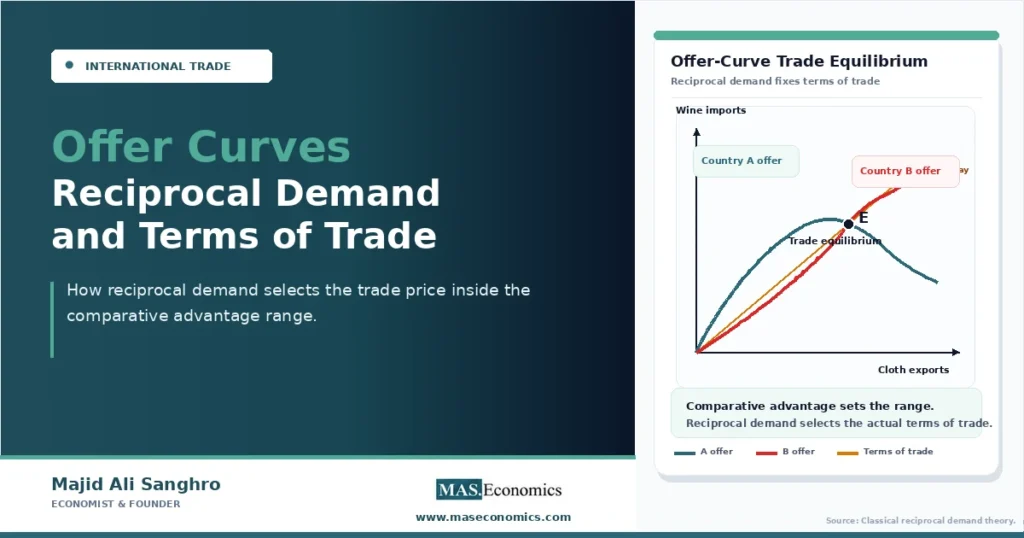
An offer curve turns this idea into geometry. It shows the combinations of exports and imports that a country would choose at different terms of trade. For Country A, the curve shows how much cloth A is willing to export in exchange for different amounts of wine. For Country B, the curve shows how much wine B is willing to export in exchange for different amounts of cloth.

The final trade equilibrium occurs where the two offer curves intersect. At that point, the quantity of cloth Country A wants to export equals the quantity of cloth Country B wants to import, and the quantity of wine Country B wants to export equals the quantity of wine Country A wants to import.

Offer curves combine supply and demand

An offer curve is sometimes called a reciprocal demand curve because it combines a country’s import demand with its export supply. It is not a standard demand curve, and it is not a standard supply curve. It is a trade curve showing willingness to exchange one good for another at alternative relative prices.

For Country A, an offer curve can be read as:

Country A Offer Curve

Here, \(X_C\) is Country A’s cloth exports and \(M_W\) is Country A’s wine imports. The curve shows the combinations A is willing to choose as the relative price of cloth changes.

For Country B, the same idea is reversed:

Country B Offer Curve

In a two-country, two-good setting, one country’s export is the other country’s import. The offer-curve intersection therefore represents mutual consistency. Each country is willing to trade exactly what the other country is willing to take at the same terms of trade.

This is why offer curves are useful in modern trade theory discussions as a bridge between classical cost-based trade and general equilibrium trade analysis. They show that trade quantities and trade prices are jointly determined.

The intersection gives equilibrium trade

The offer-curve diagram places one good on each axis. A ray from the origin represents a possible international terms-of-trade line. Its slope shows how many units of one good exchange for one unit of the other good. The equilibrium terms of trade occur where the two countries’ offer curves cross.

The economic condition at the intersection is simple:

Trade Equilibrium

At any other point, planned trades do not match. One country may want to import more than the other is willing to export, or it may want to export more than the other country is willing to absorb. The terms of trade then face pressure to adjust.

If Country A wants more wine than Country B is willing to supply at the current exchange ratio, wine becomes relatively scarce in trade. The terms of trade move in favor of wine exporters. If Country B wants more cloth than Country A is willing to supply, the terms move in favor of cloth exporters.

The equilibrium is therefore not just a quantity point. It is a price-and-quantity outcome. The intersection determines both the volume of trade and the relative price at which the exchange takes place.

Terms of trade measure the exchange

The terms of trade measure the rate at which a country’s exports exchange for its imports. A common expression is:

Commodity Terms of Trade

A higher value means export prices have risen relative to import prices.

Here, \(P_X\) is the export price index and \(P_M\) is the import price index. In an offer-curve model with two goods, the same idea appears as a relative price. The slope of the terms-of-trade ray tells how much of the import good a country receives per unit of the export good.

An improvement in the terms of trade means a country can obtain more imports for a given amount of exports. A deterioration means it must give up more exports to obtain the same amount of imports.

Offer curves show why the terms of trade can change. If a country’s demand for imports rises strongly, its offer curve may shift outward or bend in a way that makes it willing to offer more exports for imports. That can worsen its terms of trade if the trading partner’s reciprocal demand is weaker. If foreign demand for the country’s exports strengthens, the terms may improve.

Elasticity shapes bargaining strength

The elasticity of each country’s offer curve affects the distribution of gains from trade. A country with relatively inelastic demand for imports may accept less favorable terms because it strongly wants the foreign good. A country with more elastic reciprocal demand can reduce purchases more easily when the terms become unfavorable.

This does not mean a country can freely choose better terms. The terms of trade emerge from both countries’ willingness to trade. One country’s demand strength matters only in relation to the other country’s demand strength.

A simple way to read the logic is:

Table 1. Reciprocal demand and terms-of-trade pressure

Trade condition	Offer-curve implication	Terms-of-trade effect
Country A strongly demands Country B’s export	A offers more exports for imports	Terms tend to move against A
Country B strongly demands Country A’s export	B offers more exports for imports	Terms tend to move against B
Both countries have balanced reciprocal demand	Offer curves meet near the middle of the feasible range	Gains are more evenly shared
One country has weak import demand	Its offer curve is less willing to expand trade	Terms may move in its favor
Central result	Relative demand strength matters	Trade prices depend on reciprocal demand
Source: MASEconomics editorial synthesis based on classical reciprocal demand theory.

The table states the intuition, but the diagram gives the full result. A change in one country’s reciprocal demand changes the intersection of the two offer curves. That new intersection changes both trade volume and the terms of trade.

Large countries affect world prices

Offer curves are most useful when countries are large enough to affect world prices. A small country usually takes the world terms of trade as given. Its own import demand and export supply are too small to move the international exchange ratio.

A large country faces a different situation. Its demand for imports can change the world price of those imports. Its supply of exports can change the world price of those exports. In offer-curve terms, the country’s willingness to trade can move the intersection and alter the terms of trade.

This distinction also helps explain why trade policy can affect welfare differently across countries. A large country may improve its terms of trade by restricting import demand through a tariff, although such a policy can reduce world welfare and invite retaliation. A small country cannot usually shift world prices in the same way, so its tariff mostly creates domestic distortions.

The offer-curve model therefore connects reciprocal demand to broader trade-policy questions. It shows why the terms of trade are endogenous for large economies and nearly given for small economies.

Growth can shift offer curves

Economic growth changes a country’s production capacity, income, and demand for imports. These changes can shift the offer curve and alter the terms of trade. The effect depends on whether growth expands export supply, raises import demand, or changes both.

The Rybczynski theorem explains how factor growth can change output composition in a Heckscher-Ohlin setting. If growth expands production of the export good, the country may offer more exports at each terms-of-trade ratio. That can push down the relative price of its export when the country is large in world markets.

This is the logic behind the possibility of immiserizing growth. If export-biased growth causes a severe deterioration in the terms of trade, the country’s welfare gain from higher output can be offset or even reversed. That outcome is not the normal case, but offer curves make the mechanism visible.

Growth can also be import-biased. If higher income raises demand for foreign goods strongly, the country may offer more exports to obtain imports. Depending on the trading partner’s response, the terms of trade can move against the growing country.

Trade theory adds production structure

Offer curves can be drawn from a country’s production possibilities, preferences, and world price opportunities. In a full trade model, the country produces at one point, consumes at another point, and trades the difference.

The production point depends on technology and factor endowments. The consumption point depends on preferences and income at world prices. The gap between production and consumption gives exports and imports. As the world relative price changes, the production-consumption combination changes, tracing the country’s offer curve.

The Heckscher-Ohlin model adds a factor-endowment explanation for the goods a country tends to export. A capital-abundant country exports capital-intensive goods, while a labor-abundant country exports labor-intensive goods under the model’s assumptions. Offer curves then show how the quantities traded and terms of trade are determined once demand is added.

This is why offer curves should not be read as a replacement for other trade theories. They complement them. Comparative advantage explains the direction of specialization. Factor-endowment models explain why cost differences may arise. Offer curves explain how reciprocal demand helps determine the final international exchange ratio.

Diagram interpretation requires care

Offer-curve diagrams can be confusing because each country’s curve is drawn in terms of the same two goods but from opposite trade perspectives. One country’s export is the other country’s import. The axes must therefore be labeled clearly.

A common two-good diagram places Country A’s export good on the horizontal axis and Country B’s export good on the vertical axis. Country A’s offer curve shows how much of its export good it is willing to give up for imports from Country B. Country B’s offer curve shows how much of its export good it requires in exchange for imports from Country A.

The ray from the origin through the intersection gives the equilibrium terms of trade. A steeper ray means one relative price; a flatter ray means another. The welfare interpretation depends on which country exports which good.

For this reason, labels matter more than decoration. A correct offer-curve diagram should identify the two goods, the two countries, the equilibrium point, and the terms-of-trade ray. It should not overload the diagram with multiple shifts unless the article is specifically explaining comparative statics.

Offer curves have limits

The offer-curve model is powerful, but it is stylized. It usually works with two countries and two goods. It assumes clear trade balances between the two goods and abstracts from many modern features of international commerce.

Modern trade involves intermediate inputs, global value chains, firm heterogeneity, services, multinational production, exchange-rate movements, and trade policy institutions. These features are not naturally captured in the simplest offer-curve diagram.

The model also treats trade as if it were a clean exchange of goods at a relative price. In practice, trade contracts use money prices, currencies, credit, shipping costs, standards, tariffs, and legal rules. Exchange-rate movements can shift export and import prices even when underlying real trade preferences change slowly.

These limits do not make offer curves obsolete. They define the model’s proper role. Offer curves are best used to understand the theoretical determination of terms of trade under reciprocal demand, not to describe every institutional detail of modern trade.

Modern applications remain selective

Offer-curve reasoning still appears behind several modern trade ideas. Terms-of-trade effects remain central to optimal tariff theory, large-country trade policy, commodity-export dependence, and welfare analysis. The diagram is old, but the mechanism is still relevant.

For example, a commodity exporter may expand supply after a resource boom. If world demand is not elastic enough, the export price may fall relative to import prices. The country exports more physical volume but receives less import purchasing power per unit exported. That is an offer-curve-style terms-of-trade problem.

A large importer can also affect world prices. If it reduces import demand, the world price of the imported good may fall. The country may improve its terms of trade, but trading partners lose, and retaliation can reduce the gains. This is why terms-of-trade policy analysis must separate national welfare from world welfare.

Offer curves remain useful because they force trade analysis to keep two sides of the market together. Export supply and import demand are not separate stories. They are joined through the terms of trade.

Explains

Conclusion

Offer curves explain how reciprocal demand determines the terms of trade and trade volume between countries. Comparative advantage identifies the range of mutually beneficial trade, but it does not select the exact international exchange ratio. That selection occurs where each country’s willingness to export matches the other country’s willingness to import.

The offer-curve intersection is therefore a compact general-equilibrium trade result. It combines production possibilities, preferences, export supply, import demand, and relative prices in one framework. A shift in either country’s demand or supply conditions can change the terms of trade and redistribute the gains from trade.

The model is stylized, especially in a world of many goods, firms, currencies, and global value chains. Its enduring value is conceptual. It shows that trade prices are not determined by costs alone; they also depend on the reciprocal strength of demand across trading partners.

Frequently Asked Questions

Thanks for reading! If you found this helpful, share it with friends and spread the knowledge. Happy learning with MASEconomics