Total Differential Economics: Small Model Changes

A tax change, wage increase, exchange-rate movement, or price shock rarely affects only one part of an economic model. Several variables move together, and the total effect depends on all relevant marginal channels. Total differential economics gives the mathematical tool for measuring the approximate change in a function when more than one variable changes at the same time.

The total differential is the foundation of comparative statics. It turns small changes in inputs, prices, income, technology, or policy parameters into an approximate change in an economic outcome. It is simple in form, but it quietly supports many results in consumer theory, producer theory, macroeconomics, finance, and policy analysis.

The idea builds directly on differentiation. A partial derivative measures one marginal channel. A total differential combines all marginal channels into one local approximation.

Economic variables move together

Many economic outcomes depend on more than one variable. A firm’s output depends on labor and capital. A household’s utility depends on several goods. A government’s revenue depends on tax rates, income, compliance, and economic activity. A country’s export revenue depends on export prices and export quantities.

If only one variable changes, a partial derivative may be enough. If several variables change together, the total change must account for each channel. The total differential provides that accounting.

For a function with two variables:

Two-variable function

The outcome \(z\) depends on both \(x\) and \(y\).

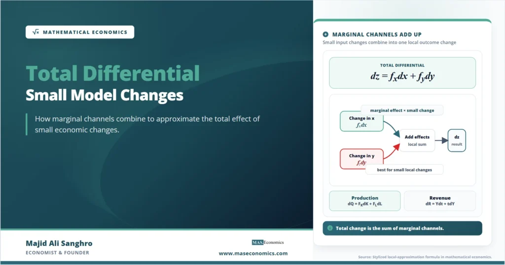
A small change in \(x\) and \(y\) produces an approximate change in \(z\):

Total differential

Each partial derivative measures one marginal channel, and each differential measures the small change in that variable.

The formula says that the total effect is the sum of the separate marginal effects. The effect of \(x\) is \(f_x dx\). The effect of \(y\) is \(f_y dy\). Added together, they give the local change in the outcome.

Partial derivatives become components

A partial derivative isolates one channel. In \(z=f(x,y)\), the partial derivative \(f_x\) measures how \(z\) changes when \(x\) changes while \(y\) is held constant. The partial derivative \(f_y\) does the same for \(y\).

The total differential does not replace partial derivatives. It uses them. Each partial derivative becomes one component of the total change.

Component effects

This is why the notation is useful in economics. A price effect, income effect, technology effect, and policy effect can be separated before being recombined. The total differential keeps the mechanism transparent.

For small changes, this approximation is usually accurate enough for local comparative statics. For large changes, the approximation may become less reliable because slopes can change as the variables move.

The formula generalizes cleanly

For a function with many variables:

Many-variable function

The total differential is:

General total differential

In compact notation:

The structure is the same as the two-variable case. Each variable has a marginal effect and a small change. The total differential multiplies each marginal effect by its corresponding change and adds the results.

This form is especially useful in economic models because the number of variables can grow quickly. Instead of writing every channel in prose, the formula gives a disciplined way to track the local effect of simultaneous changes.

A production example shows intuition

Consider a production function:

Production function

Output \(Q\) depends on capital \(K\) and labor \(L\).

The total differential is:

Output change

Here, \(F_K\) is the marginal product of capital, and \(F_L\) is the marginal product of labor. The term \(F_KdK\) measures the output change from a small increase in capital. The term \(F_LdL\) measures the output change from a small increase in labor.

If capital rises while labor falls, the two terms may move in opposite directions. Output can rise, fall, or remain nearly unchanged depending on the relative size of the marginal products and the changes in inputs.

This makes the total differential useful for production analysis. It can explain why a firm’s output may rise only slightly even after investment if labor declines at the same time, or why employment growth may have a larger effect when capital is already abundant.

A revenue example adds policy meaning

Government revenue from a proportional tax can be written as:

Tax revenue

Revenue \(R\) depends on the tax rate \(t\) and taxable income \(Y\).

The total differential is:

Revenue change

The first term, \(Ydt\), is the direct effect of changing the tax rate. The second term, \(tdY\), is the effect of a change in the tax base. This separation is valuable because a tax-rate increase does not guarantee a proportional increase in revenue if taxable income changes at the same time.

For example, if \(t=0.20\), \(Y=1{,}000\), \(dt=0.01\), and \(dY=-20\), then:

The tax-rate effect raises revenue by 10 units, while the smaller tax base reduces revenue by 4 units. The approximate total revenue gain is 6 units.

This example shows the practical value of the total differential. It separates direct policy effects from indirect economic responses.

The visual logic is local

The total differential is a local approximation. It uses the slope of the function near the starting point to estimate the effect of small changes. It does not redraw the entire function.

The diagram shows the main logic. Each small variable change contributes one component to the total effect. The total differential adds those components to approximate the change in the outcome.

Comparative statics uses differentials

Comparative statics studies how equilibrium outcomes change after a parameter changes. Total differentials make this possible when the model is written as an equation rather than an explicit solution.

Consider an equilibrium condition:

Equilibrium condition

The endogenous variable \(x\) adjusts when the parameter \(a\) changes.

The total differential is:

Solving for the local response gives:

Comparative-static derivative

This formula is used throughout economic theory. It shows how an equilibrium variable responds to a small parameter change while the equilibrium condition remains satisfied.

The denominator \(F_x\) measures the local restoring force. If \(x\) strongly affects the equilibrium condition, only a small change in \(x\) is needed. If \(x\) weakly affects the condition, the same shock may require a large adjustment.

Chain rules require total effects

Total differentials also clarify the chain rule. Suppose output depends on capital and labor, but capital and labor both depend on time:

The total change in output over time is:

Total derivative over time

This is a total derivative, built from the same logic as the total differential. Output changes because capital changes and labor changes. Each channel is weighted by its marginal product.

This distinction matters in growth, production, and macroeconomic models. A change in time, policy, technology, or income may affect several intermediate variables, and those variables jointly affect the final outcome.

Elasticities are related approximations

Total differentials are often converted into percentage changes. This is especially useful when economists want to compare effects measured in different units.

For a function \(Y=F(K,L)\), dividing the total differential by \(Y\) gives:

Proportional approximation

The terms \(\frac{F_KK}{Y}\) and \(\frac{F_LL}{Y}\) are elasticities or shares in many economic settings. They show how sensitive output is to proportional changes in capital and labor.

For a Cobb-Douglas production function:

The proportional differential is:

Cobb-Douglas percentage change

This expression shows why total differentials matter in growth accounting. Output growth can be decomposed into technology growth, capital growth, and labor growth.

Exact and approximate changes differ

The total differential is exact as a differential expression, but it is an approximation when used to estimate finite changes. The approximation works best when changes are small and the function is smooth near the starting point.

For a small finite change, economists often write:

Linear approximation

The symbol \(\approx\) matters. It signals that the expression estimates the change using local slopes. If the function is highly curved or the change is large, the approximation may miss important second-order effects.

For example, if marginal cost rises sharply with output, a small output increase may be well approximated by the current marginal cost. A large output increase requires accounting for the fact that marginal cost itself changes as output expands.

This is why total differentials often sit beside Hessian analysis in mathematical economics. First derivatives give the local linear effect. Second derivatives describe how those local effects change as the model moves away from the starting point.

A table separates common uses

The same total-differential logic appears in many economic settings, but each setting gives the terms a different interpretation.

Table 1. Total differentials in economic models

Model setting	Total differential form	Economic interpretation
Production	\(dQ=F_KdK+F_LdL\)	Output changes through capital and labor channels
Utility	\(dU=U_xdx+U_ydy\)	Utility changes through marginal utilities and consumption changes
Tax revenue	\(dR=Ydt+tdY\)	Revenue changes through tax-rate and tax-base channels
Equilibrium	\(F_xdx+F_ada=0\)	Endogenous variables adjust to keep equilibrium conditions true
Growth accounting	\(\frac{dY}{Y}=\frac{dA}{A}+\alpha\frac{dK}{K}+\beta\frac{dL}{L}\)	Output growth is decomposed into productivity and input growth
Central rule	Marginal effect × small change	Total change is built from component channels
Source: MASEconomics editorial synthesis based on standard mathematical economics notation.

The table shows why the total differential is not limited to one field. It is a general method for decomposing local change in economic models.

Holding constant changes the meaning

Partial derivatives require holding other variables constant. Total differentials allow those other variables to change. Confusing the two can lead to wrong economic conclusions.

For example, \(\partial Q/\partial L\) measures the marginal product of labor holding capital constant. The total change \(dQ\) allows both labor and capital to move. If labor rises but capital falls, the total output effect may be smaller than the labor partial derivative suggests.

The same issue appears in demand analysis. A partial price effect holds income constant. A total effect may include income changes, related price changes, or policy changes. The interpretation depends on which variables are allowed to move.

This is why notation matters. The symbol \(\partial\) signals a partial effect. The symbol \(d\) signals a total differential or total change along a specified path.

Local paths matter economically

A total differential depends on the path of change. If \(x\) and \(y\) both change, the final local effect depends on the relative size and direction of \(dx\) and \(dy\).

In a utility function, a consumer may gain utility from more of one good but lose utility from less of another. In a production function, more capital and less labor can offset each other. In a macroeconomic model, higher government spending and higher interest rates can push output in opposite directions.

The total differential makes these trade-offs explicit. It does not hide opposing forces behind a single net result. Each channel remains visible before the final effect is summed.

This is especially useful for policy analysis. A policy can have a direct positive effect and an indirect negative effect. The total differential helps organize those effects in one expression.

Second-order terms limit accuracy

The total differential is a first-order approximation. It uses the first derivatives evaluated at a point. The omitted part of a finite-change approximation comes from curvature and higher-order terms.

For two variables, a second-order Taylor approximation adds curvature terms:

Second-order extension

The first two terms are the total differential. The remaining terms account for curvature. When changes are tiny, squared terms are usually small. When changes are large, curvature may matter.

This explains why total differentials are powerful but limited. They are excellent for local reasoning and small comparative-static changes. They are not designed to capture large nonlinear transitions by themselves.

Economic modeling uses them constantly

Total differentials appear throughout economic modeling because they make change analyzable. They are used in consumer theory to decompose utility changes, in producer theory to decompose output changes, and in macroeconomics to derive multipliers.

They are also central in finance. A bond price can be approximated using duration and yield changes. A portfolio value can be approximated using sensitivities to interest rates, exchange rates, and asset prices. Each term in the total differential represents one risk channel.

In international economics, export revenue changes through price and quantity. If \(R=P_X X\), then:

This separates price effects from quantity effects. A country can export more and still see revenue fall if the price effect is negative enough. The same logic appears in terms-of-trade analysis, commodity markets, and trade-welfare models.

Explains

Conclusion

Total differential economics explains how small changes in several variables combine to change an economic outcome. It takes partial derivatives, weights them by small variable changes, and adds them into one local approximation.

The method is central because economic variables rarely move one at a time. Output changes through labor, capital, and technology. Revenue changes through rates and bases. Equilibrium changes through shocks and adjustment forces. Total differentials provide the notation and logic for tracking those channels clearly.

The result is local, not global. It is strongest for small changes around a known point and smooth functions. When shocks are large, or curvature is strong, second-order terms and broader model analysis become necessary.

Frequently Asked Questions

Did you find this article helpful? Share it with someone who loves economics. And remember, at MASEconomics, we make complex ideas simple.