How to Detect and Correct Heteroscedasticity in Econometric Models

Heteroscedasticity is a common issue in econometric analysis, particularly when dealing with cross-sectional data or financial time series. It refers to the situation where the variance of the error terms in a regression model is not constant across observations, which violates one of the key assumptions of the classical linear regression model. If not addressed properly, this can lead to inefficient estimates and invalid statistical inferences. In this post, we will delve into the following key aspects of heteroscedasticity:

• What is heteroscedasticity, and its impact on regression analysis?

• Methods to detect heteroscedasticity, including graphical methods and formal tests.

• Approaches to correct heteroscedasticity to ensure reliable results.

What is Heteroscedasticity?

In a classical linear regression model, one key assumption is that the error terms variance (denoted as 𝜀) is constant, a property known as homoscedasticity. When this assumption is violated, and the variance of the errors changes depending on the level of an independent variable, the errors are said to be heteroscedastic. This means that some observations have greater variability than others, and this variation is often systematic, depending on the level of the predictor variable.

\[ E(\epsilon_i^2 \mid X) = \sigma_i^2 \]

• \( \sigma_i^2 \) varies with the values of \( X \), the independent variable(s).

Heteroscedasticity often arises in data where there is a wide variation in the magnitude of the dependent variable for different levels of the independent variable. For example, in studies on income and consumption, wealthier households tend to have more variability in consumption than poorer households, leading to heteroscedastic errors. Other examples include financial data, where volatility increases as market returns increase, and environmental studies, where the impact of pollution levels may vary by region.

Impact on Regression Analysis

Heteroscedasticity directly impacts the efficiency and reliability of the Ordinary Least Squares (OLS) estimator. While OLS estimates remain unbiased, meaning they are still centered around the true value, they lose the property of being efficient when heteroscedasticity is present. This means that OLS is no longer the Best Linear Unbiased Estimator (BLUE), as it fails to have the smallest variance among unbiased estimators.

Key Consequences of Heteroscedasticity:

Inefficient Estimates

The presence of heteroscedasticity inflates the variance of the coefficients, leading to larger standard errors. This makes it harder to precisely estimate the relationship between variables, affecting the accuracy of the model’s predictions.

Biased Standard Errors

The estimated standard errors of the coefficients will be biased when heteroscedasticity exists, resulting in invalid hypothesis tests. As a result, t-tests, F-tests, and confidence intervals are no longer reliable, which can mislead researchers into either accepting or rejecting hypotheses incorrectly.

Suboptimal Policy and Business Decisions

In real-world applications like economic forecasting or financial risk management, heteroscedasticity can lead to suboptimal decisions. For example, policymakers might underestimate the impact of fiscal policies on inflation, or businesses might misjudge market trends based on faulty econometric models.

In summary:

• Unbiasedness: OLS estimators remain unbiased.

• Efficiency Loss: OLS estimators lose efficiency, leading to larger variances than necessary.

• Hypothesis Testing: The standard errors of OLS estimates are biased, invalidating hypothesis tests.

Given these significant consequences, it’s important to detect heteroscedasticity early in your regression analysis and apply appropriate corrections.

Methods to Detect Heteroscedasticity

There are several ways to detect heteroscedasticity, including both graphical methods and formal statistical tests. These techniques help in identifying whether the variability of the error terms changes with the independent variable(s).

Graphical Methods

One of the simplest ways to detect heteroscedasticity is through graphical analysis. After fitting an OLS regression model, you can plot the residuals (the difference between actual and predicted values of the dependent variable) against the predicted values or the independent variable(s). If the variance of the residuals increases or decreases systematically with the predicted values, this indicates heteroscedasticity.

Example: Plotting Residuals

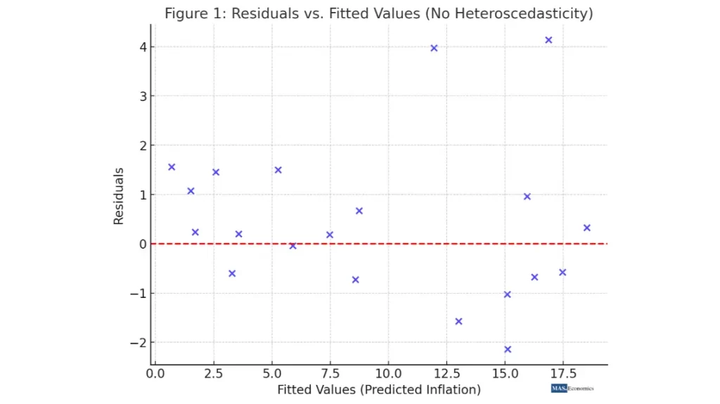
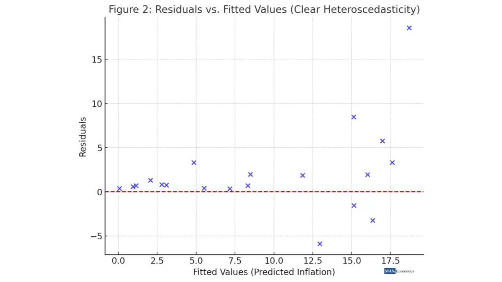
Let’s consider a model predicting inflation using GDP growth. After fitting the OLS regression, you plot the residuals against predicted values of inflation. If the residuals “fan out” or show a pattern where the spread increases as predicted inflation rises, this is a sign of heteroscedasticity.

Here is the scatter plot of residuals vs. fitted values, illustrating no heteroscedasticity. In this case, the residuals appear to be randomly scattered around zero without a clear pattern, indicating no signs of heteroscedasticity. The red dashed line represents the zero residual line, and as seen, the residuals don’t fan out or shrink as the predicted values increase, confirming the absence of heteroscedasticity.

Here is the scatter plot of residuals vs. fitted values, showing clear heteroscedasticity. In this case, the residuals exhibit a fanning-out pattern, with larger predicted values associated with a wider spread of residuals. This pattern suggests that the variance of errors increases with the predicted values, a classic indication of heteroscedasticity.

Graphical methods offer a quick and intuitive way to spot heteroscedasticity, but they are not foolproof. For more rigorous analysis, formal statistical tests are often necessary.

Formal Tests for Heteroscedasticity

Several statistical tests can help formally detect heteroscedasticity:

Breusch-Pagan Test

The Breusch-Pagan test is one of the most widely used tests for detecting heteroscedasticity. It tests whether the variance of the residuals is related to the independent variables. The steps are as follows:

1. Estimate the OLS regression and obtain the residuals.
2. Regress the squared residuals on the independent variables.
3. The null hypothesis is that the coefficients of the independent variables in this auxiliary regression are all zero, meaning no heteroscedasticity.

The Breusch-Pagan test statistic follows a chi-square distribution. If the test statistic is large, the null hypothesis of homoscedasticity is rejected, indicating heteroscedasticity.

White Test

The White test is more general than the Breusch-Pagan test and doesn’t require specifying a particular form of heteroscedasticity. Instead, it tests whether the variance of the residuals is related to independent variables, their squares, or interaction terms.

Steps:

1. Estimate the OLS regression and obtain the residuals.
2. Regress the squared residuals on the independent variables, their squares, and interaction terms.
3. The test statistic, based on the R-squared from this auxiliary regression, follows a chi-square distribution.

Goldfeld-Quandt Test

This test is particularly useful when heteroscedasticity is believed to be related to one independent variable. The data is divided into two subsets, one with lower values and one with higher values of the independent variable suspected of causing heteroscedasticity. The residuals from both subsets are compared.

Steps:

1. Order the data based on the suspected variable.
2. Split the data into two groups and estimate separate OLS regressions for each group.
3. Compare the residual sum of squares using an F-test.

Correcting for Heteroscedasticity

Once heteroscedasticity is detected, several methods can correct it, ensuring more accurate and reliable results from your regression analysis. The choice of correction method depends on the nature of the heteroscedasticity and the model you’re using.

Weighted Least Squares (WLS)

One way to handle heteroscedasticity is to use Weighted Least Squares (WLS). WLS adjusts the regression model by assigning a weight to each observation, which is inversely proportional to its variance. This corrects for the unequal variance and ensures the model fits all observations equally well.

In the transformed model:

\[ \frac{Y_i}{\sigma_i} = \alpha + \beta \frac{X_i}{\sigma_i} + \frac{\epsilon_i}{\sigma_i} \] Where \( \sigma_i \) represents the standard deviation of the errors. This transformation makes the variance of the errors constant (homoscedastic), allowing the use of OLS.

Robust Standard Errors (Huber-White)

If transforming the model is not ideal, you can use heteroscedasticity-robust standard errors, also known as Huber-White standard errors. This method doesn’t change the model but adjusts the standard errors to account for heteroscedasticity, ensuring valid hypothesis tests and more reliable confidence intervals.

Generalized Least Squares (GLS)

A more sophisticated approach is Generalized Least Squares (GLS). Like WLS, it transforms the model so that the error variances become constant. However, GLS goes further by using a transformation matrix that adjusts the model more comprehensively, ensuring efficiency even when complex heteroscedastic patterns are present.

Practical Example: Analyzing Inflation Volatility

To make these concepts more tangible, let’s walk through a practical example. Consider an econometrician who wants to analyze the relationship between inflation volatility, GDP growth, and unemployment rates. Inflation volatility will likely vary more at higher GDP growth rates, leading to heteroscedastic errors.

Here are the steps:

1. Fit an OLS regression model with inflation as the dependent variable and GDP growth and unemployment as the independent variables.
2. Use graphical methods to check for heteroscedasticity by plotting the residuals against predicted inflation values.
3. Perform a Breusch-Pagan test to formally confirm the presence of heteroscedasticity.
4. If heteroscedasticity is detected, correct for it using robust standard errors or GLS.

By addressing heteroscedasticity, the model becomes more accurate, allowing for better predictions and a more informed economic analysis.

Conclusion

Heteroscedasticity, if left unaddressed, can severely impact the reliability of econometric models. Detecting it early through graphical methods and formal tests ensures that your analysis remains robust. Moreover, applying corrective measures such as Weighted Least Squares (WLS), robust standard errors, or Generalized Least Squares (GLS) enables econometricians to obtain efficient estimates and valid hypothesis tests.

In the next post, we will tackle another common econometric issue—autocorrelation—and explore how it can affect time series models. Stay tuned!

FAQs:

What is heteroscedasticity in econometric models?

Heteroscedasticity refers to a condition where the variance of the error terms in a regression model is not constant across observations. This violates the homoscedasticity assumption of the classical linear regression model, leading to inefficient estimates and unreliable statistical inferences.

How does heteroscedasticity impact regression analysis?

Heteroscedasticity affects regression analysis by inflating the variance of coefficient estimates, making them less precise. It can also result in biased standard errors, leading to invalid t-tests, F-tests, and confidence intervals, which can misguide hypothesis testing.

What are some methods to detect heteroscedasticity?

You can detect heteroscedasticity using graphical methods like plotting residuals against predicted values, as well as formal tests such as the Breusch-Pagan test, the White test, and the Goldfeld-Quandt test.

How do you correct heteroscedasticity in a regression model?

Common methods to correct heteroscedasticity include using Weighted Least Squares (WLS), applying heteroscedasticity-robust standard errors (Huber-White), or using Generalized Least Squares (GLS) to adjust the model for varying error variances.

Why is it important to address heteroscedasticity in econometric models?

Addressing heteroscedasticity ensures that your regression model produces efficient and reliable estimates, allowing for valid hypothesis tests and accurate economic predictions. This is crucial for making informed policy and business decisions based on the model’s results.

Thanks for reading! If you found this helpful, share it with friends and spread the knowledge.
Happy learning with MASEconomics