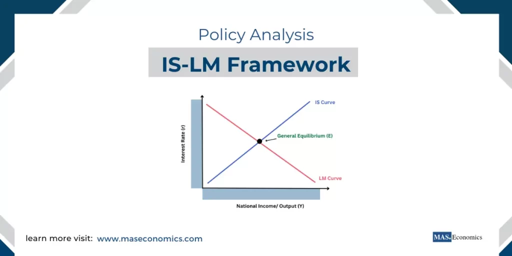
The IS-LM framework is a foundational model in macroeconomics used to analyze the interaction between the real economy and the money market. Developed by John Hicks and Alvin Hansen, it combines the Investment-Saving (IS) curve and the Liquidity Preference-Money Supply (LM) curve to determine equilibrium in both the goods and money markets. The IS-LM framework helps us understand how different policies—both fiscal and monetary—affect aggregate demand, income, interest rates, and ultimately, economic activity.
In this article, we’ll explore the IS-LM model in depth, including how it is constructed, how it responds to different shocks, and its implications for policy analysis. We will also illustrate how governments and central banks use the IS-LM framework to make real-time decisions and maintain economic stability.
Understanding the IS Curve
The IS curve represents the equilibrium in the goods market, where aggregate demand equals aggregate supply. It shows the relationship between income (Y) and the interest rate (r) that ensures equilibrium in the goods market. The IS curve is derived from the following equation for aggregate demand:
Where \(C\) represents consumption, which includes all spending by households on goods and services; \(I\) represents investment, referring to spending by businesses on capital goods and inventories that support future production; \(G\) stands for government spending, which is the expenditure by the government on goods and services to provide public utilities; and \(NX\) represents net exports, which is the difference between exports and imports, capturing the impact of trade on aggregate demand.
The level of investment (\(I\)) depends negatively on the interest rate, as higher interest rates increase the cost of borrowing, thereby reducing investment. This inverse relationship between the interest rate and aggregate demand gives the IS curve its negative slope. Essentially, as interest rates decrease, investment and consumption rise, leading to higher levels of income, which shifts the economy to a higher equilibrium point.
Consider a scenario where the government decides to increase spending (\(G\)). This fiscal stimulus will increase aggregate demand, causing the IS curve to shift to the right, indicating higher equilibrium income at any given interest rate. The shift in the IS curve captures the multiplier effect, where an initial increase in spending leads to multiple rounds of increased consumption and income.
Understanding the LM Curve
The LM curve represents the equilibrium in the money market. It shows the combinations of income (Y) and interest rate (r) for which the demand for money equals the supply of money. The LM curve is derived from the liquidity preference theory, which explains how individuals decide to hold their wealth in the form of money or bonds, depending on the interest rate.
The equation for money demand is typically represented as follows:
Where \(M^d\) represents money demand, and \(L(Y, r)\) represents the liquidity preference function, which depends positively on income (\(Y\)) and negatively on the interest rate (\(r\)). The higher the income level, the greater the transactions demand for money, which leads to a positive relationship between income and money demand. On the other hand, the interest rate influences the opportunity cost of holding money rather than interest-bearing assets like bonds—thus, higher interest rates reduce the demand for money as individuals prefer to invest in these assets.
The supply of money (\(M^s\)) is determined by the central bank. The LM curve represents the combinations of interest rates and income where money demand equals money supply. An increase in income leads to an increase in the demand for money, putting upward pressure on interest rates, which is why the LM curve is upward-sloping.
If the central bank decides to increase the money supply, the LM curve shifts to the right, leading to lower interest rates for any given level of income. This shift demonstrates how monetary policy can be used to influence economic activity by making borrowing cheaper and stimulating investment and consumption.
Equilibrium in the IS-LM Model
The intersection of the IS and LM curves represents the general equilibrium in both the goods and money markets. The equilibrium point provides the equilibrium level of income (Y) and the equilibrium interest rate (r). The IS-LM model allows us to analyze the effects of different types of economic policies—fiscal policy (shifts in the IS curve) and monetary policy (shifts in the LM curve)—on the overall economy.
To visualize this concept better, consider the diagram below showing General Equilibrium in the IS-LM Framework:
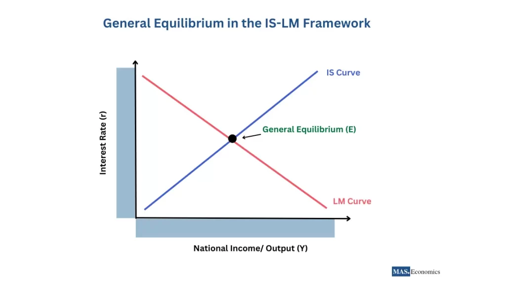
In the diagram above, the IS curve (in blue) and the LM curve (in red) intersect at point E, which represents the general equilibrium of the economy. As seen in the diagram, this equilibrium determines the combination of the interest rate () and national income () at which both the goods market and the money market are simultaneously in balance. The visual representation of these curves helps to illustrate how different policy interventions shift these curves and impact equilibrium outcomes.
For example, consider the impact of an expansionary monetary policy, such as an increase in the money supply. This policy shifts the LM curve to the right, leading to a lower interest rate. The lower interest rate, in turn, stimulates investment, which results in higher aggregate demand and increased equilibrium income. This process illustrates the power of monetary policy in stabilizing the economy, particularly during periods of recession.
Conversely, an expansionary fiscal policy, such as increased government spending, shifts the IS curve to the right. This increases income and, due to higher demand for money, also puts upward pressure on the interest rate. If capital is relatively immobile, the increase in interest rates may not significantly deter investment, making fiscal policy highly effective in stimulating aggregate demand.
Shocks and Dynamic Adjustments in the IS-LM Model
In the real world, economies are often subject to demand shocks and supply shocks that can impact equilibrium. The IS-LM model can be used to analyze how these shocks affect economic activity and what role policy can play in mitigating their effects.
Demand Shocks, such as an increase in consumer confidence or a surge in government spending, shift the IS curve to the right, increasing both income and interest rates. Governments may use monetary policy to counterbalance the impact of rising interest rates by increasing the money supply and shifting the LM curve to the right to maintain economic stability.
Supply Shocks, such as a sudden increase in oil prices, can have a more complex impact. An oil price shock typically increases production costs, leading to higher prices and potentially lower aggregate supply. The IS-LM framework can be extended by incorporating the aggregate supply (AS) curve to understand how such shocks affect both output and inflation. Policymakers may face difficult trade-offs in responding to supply shocks, as expansionary policies aimed at supporting output may lead to higher inflation.
Policy Analysis Using the IS-LM Framework
The IS-LM model is a powerful tool for policy analysis, as it helps to illustrate the trade-offs involved in using fiscal and monetary policies. For example, during a recession, the government might implement an expansionary fiscal policy, such as increased infrastructure spending. This policy shifts the IS curve to the right, leading to higher equilibrium income. However, the resulting increase in interest rates could crowd out private investment unless the central bank also enacts an accommodative monetary policy to keep interest rates low.
The effectiveness of these policies depends on the degree of capital mobility and the type of exchange rate regime in place. Under a fixed exchange rate regime, monetary policy loses some of its effectiveness because the central bank must intervene in the foreign exchange market to maintain the fixed exchange rate, often limiting its ability to adjust the money supply freely. In contrast, under a flexible exchange rate regime, monetary policy becomes more powerful, as changes in interest rates directly affect exchange rates and, by extension, net exports.
Practical Case Studies
Let’s look at some practical examples of how governments and central banks use the IS-LM framework in real-time decision-making. Many governments implemented expansionary fiscal policies during the 2008 global financial crisis to boost aggregate demand. The United States, for instance, passed the American Recovery and Reinvestment Act (ARRA), which increased government spending and shifted the IS curve to the right. Simultaneously, the Federal Reserve pursued an expansionary monetary policy, lowering interest rates and using quantitative easing to increase the money supply, shifting the LM curve to the right. These combined measures aimed to restore equilibrium at a higher level of income and lower interest rates, helping the economy recover more quickly.
Another example is the European Central Bank (ECB) during the Eurozone debt crisis. In response to falling aggregate demand and rising unemployment, the ECB increased the money supply, which shifted the LM curve to the right and lowered interest rates across the Eurozone. However, due to differences in fiscal capacity across member countries, the effectiveness of these policies varied, highlighting the importance of coordinated fiscal and monetary responses.
The IS-LM Framework in an Open Economy Context
The IS-LM model can also be extended to analyze open economies, where trade and capital flows play significant roles. In an open economy, the IS curve is affected not only by domestic consumption, investment, and government spending but also by net exports. Exchange rates play a critical role in determining net exports, and thus shifts in the IS curve can be influenced by changes in the exchange rate.
The Mundell-Fleming model, which builds on the IS-LM framework, helps to explain how macroeconomic policies work in open economies with different levels of capital mobility and exchange rate regimes. For instance, in an open economy with a fixed exchange rate, fiscal policy is highly effective, as it increases income without causing an appreciation in the exchange rate. In contrast, monetary policy is more effective under a flexible exchange rate, where changes in interest rates influence the exchange rate, which in turn affects net exports.
Dynamic Adjustments to Shocks: Demand vs. Supply Shocks
The IS-LM framework also provides insights into how the economy dynamically adjusts to various shocks. Consider a demand shock such as a government stimulus. When the IS curve shifts to the right, both income and interest rates rise. The higher interest rate might reduce investment unless the central bank intervenes to increase the money supply. The central bank can shift the LM curve to the right, bringing interest rates back down and supporting the higher level of aggregate demand.
In the case of a supply shock, such as an increase in oil prices, the IS-LM framework alone is insufficient to capture the full dynamics, as the aggregate supply curve must also be considered. A negative supply shock will raise production costs, reduce output, and increase prices. In such a scenario, policymakers face a dilemma—supporting output through expansionary policies may exacerbate inflation, whereas contractionary policies to contain inflation may lead to a deeper recession.
Conclusion
The IS-LM framework is a versatile tool for understanding the interactions between the real economy and the money market, as well as for analyzing the effects of fiscal and monetary policies. By combining the goods market (IS) and money market (LM) relationships, the model provides valuable insights into how equilibrium income and interest rates are determined, and how different shocks and policies can influence the economy.
Incorporating both real-world case studies and dynamic adjustments to shocks helps illustrate the practical importance of the IS-LM model for policymakers. From managing economic recessions to stabilizing financial crises, the IS-LM model remains a critical framework for understanding the trade-offs and complexities involved in macroeconomic policy-making.
FAQs:
What is the IS-LM framework?
The IS-LM framework is a macroeconomic model that combines the IS curve (Investment-Saving) representing the goods market equilibrium with the LM curve (Liquidity Preference-Money Supply) representing the money market equilibrium. It helps explain how interest rates and income levels are determined in an economy. The model shows how fiscal and monetary policies influence aggregate demand, income, and interest rates.
How does the IS curve represent the goods market?
The IS curve shows the relationship between income (Y) and interest rates (r) where the goods market is in equilibrium—where total spending matches total output. It is downward sloping, indicating that lower interest rates encourage higher investment, increasing income. For example, an increase in government spending shifts the IS curve to the right, boosting income at every interest rate level.
What does the LM curve represent?
The LM curve represents equilibrium in the money market, showing combinations of income (Y) and interest rates (r) where money demand equals money supply. It is upward-sloping because higher income leads to increased demand for money, which puts upward pressure on interest rates. For example, an increase in the money supply shifts the LM curve to the right, lowering interest rates and encouraging investment.
How do fiscal and monetary policies impact the IS-LM framework?
- Fiscal policy, such as increased government spending or tax cuts, shifts the IS curve to the right, raising both income and interest rates.
- Monetary policy, like increasing the money supply, shifts the LM curve to the right, reducing interest rates and raising income.
These policies can complement each other—monetary easing can offset the rise in interest rates from fiscal expansion, preventing crowding out of private investment.
What is the equilibrium in the IS-LM model?
The equilibrium is where the IS and LM curves intersect, representing the point where both the goods and money markets are in balance. At this point, we determine the economy’s equilibrium income and interest rate. Changes in fiscal or monetary policy shift the curves and alter the equilibrium, allowing policymakers to influence economic output and borrowing costs.
How does the IS-LM framework explain demand and supply shocks?
- Demand shocks, such as increased consumer confidence or government spending, shift the IS curve to the right, raising income and interest rates. Policymakers can respond with monetary easing to keep interest rates low and support investment.
- Supply shocks, like rising oil prices, reduce output and increase inflation. These shocks pose policy dilemmas since supporting output with fiscal or monetary expansion may worsen inflation.
What are the policy trade-offs in the IS-LM model?
The IS-LM framework highlights trade-offs in policy-making. For example, fiscal expansion raises income but can increase interest rates, potentially crowding out private investment. Monetary policy can offset this by lowering interest rates, but excessive monetary easing risks inflation. Policymakers must carefully balance these trade-offs to ensure sustainable growth.
How does the IS-LM model function in an open economy?
In an open economy, the IS-LM framework is extended through the Mundell-Fleming model, which considers exchange rates and international capital flows. Under a fixed exchange rate, fiscal policy is more effective because it doesn’t lead to currency appreciation. Under a flexible exchange rate, monetary policy is more powerful since changes in interest rates affect exchange rates and net exports.
Can the IS-LM framework address financial crises?
Yes, the IS-LM model helps explain how fiscal and monetary policies stabilize economies during crises. For example, during the 2008 financial crisis, the U.S. government implemented fiscal stimulus (shifting the IS curve right), while the Federal Reserve lowered interest rates through monetary easing (shifting the LM curve right). This combination helped restore growth and prevent deeper economic contraction.
What are the limitations of the IS-LM framework?
The IS-LM model simplifies the economy by assuming fixed prices and focusing on short-term equilibrium. It doesn’t fully capture inflation dynamics or global financial flows, limiting its applicability during periods of high inflation or in highly interconnected economies. Despite these limitations, it remains a useful tool for understanding how policies affect output, interest rates, and aggregate demand.
Thanks for reading! Share this with friends and spread the knowledge if you found it helpful.
Happy learning with MASEconomics

