Autocorrelation is a significant issue in time series econometrics, one that can greatly affect the accuracy and reliability of econometric models. In simple terms, autocorrelation occurs when the residuals (errors) of a regression model are correlated with one another over time. This is a common issue in time series data because, unlike cross-sectional data, observations taken at different points in time are often influenced by prior observations. Therefore, detecting and correcting for autocorrelation is essential for obtaining reliable and valid estimates in time series econometric models.
In this post, we will cover:
- What autocorrelation is and its causes
- How autocorrelation affects time series models
- Methods to detect and correct autocorrelation, such as the Durbin-Watson test
- A practical example of conducting autocorrelation analysis
What is Autocorrelation?
Autocorrelation refers to the correlation between the values of a variable at different points in time. In econometric models, particularly time series models, autocorrelation occurs when the residuals (or errors) of a regression model are correlated across time. This violates one of the classical assumptions of linear regression—that residuals should be independent of each other.
Mathematically, autocorrelation at lag \( k \) is given by the following formula:- \( \rho_k \) is the autocorrelation coefficient at lag \( k \),
- \( Cov(Y_t, Y_{t-k}) \) is the covariance between \( Y_t \) and its value at a previous time period \( t – k \),
- \( Var(Y_t) \) is the variance of \( Y_t \).
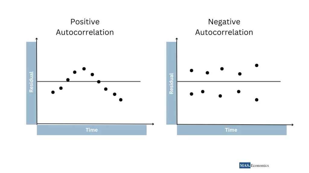
Autocorrelation can be either positive or negative. In the case of positive autocorrelation, residuals tend to have the same sign over time, i.e., positive errors follow positive errors and negative errors follow negative errors. On the other hand, negative autocorrelation occurs when residuals alternate in sign, meaning that positive residuals are followed by negative residuals, and vice versa.
Causes of Autocorrelation
Autocorrelation in time series data can arise for several reasons:
Data Smoothing or Interpolation
In cases where time series data has been smoothed or interpolated, the resulting series may exhibit autocorrelation due to the smoothing process itself.
Omitted Variables
If important explanatory variables are left out of the regression model, their effects may be captured in the residuals, leading to autocorrelation. In time series data, omitting relevant lagged variables can often cause this issue.
Model Misspecification
Incorrect model specifications can lead to autocorrelation. For instance, if a linear model is fitted to data with a nonlinear relationship, autocorrelation can arise.
Lagged Effects
Time series data is often influenced by past values of the variables. For instance, a firm’s stock price today is likely affected by its price yesterday, which can create autocorrelation in the residuals.
Data Smoothing or Interpolation
In cases where time series data has been smoothed or interpolated, the resulting series may exhibit autocorrelation due to the smoothing process itself.
Effects of Autocorrelation on Time Series Models
Autocorrelation has several adverse effects on time series models, particularly those estimated using the Ordinary Least Squares (OLS) method:
Inefficient Estimates
While OLS estimates remain unbiased in the presence of autocorrelation, they are no longer efficient. This means that the estimates do not have the minimum possible variance, which results in less precise parameter estimates.
Invalid Hypothesis Testing
The standard errors of the estimated coefficients become biased when autocorrelation is present, leading to inaccurate hypothesis tests. For example, t-tests and F-tests may suggest statistical significance when none exists, or they may fail to detect a significant relationship, leading to either Type I or Type II errors.
Overestimated R squared
Positive autocorrelation can inflate the R2 statistic, giving the misleading impression that the model fits the data better than it actually does. This false sense of accuracy can lead to overconfidence in the model’s predictive power.
Misleading Forecasts
In practice, if a model suffers from autocorrelation, its forecasts and policy recommendations may be unreliable. For instance, central banks or financial institutions could misjudge economic conditions if their econometric models fail to account for autocorrelation in key indicators like inflation or interest rates.
Detecting Autocorrelation
Detecting autocorrelation is a crucial step in any time series econometric analysis. Several methods can be used, ranging from simple graphical techniques to more formal statistical tests.
Graphical Methods: Residual Plots
One of the simplest ways to detect autocorrelation is by visually inspecting a plot of the residuals over time. If residuals show a pattern, such as a wave-like form or clusters of residuals with the same sign, this is often a sign of autocorrelation.
Let’s consider a model estimating GDP growth. By plotting the residuals against time, we notice that periods of positive residuals are followed by more positive residuals, while periods of negative residuals tend to be followed by more negative residuals. This pattern signals positive autocorrelation.

The figure 1 illustrates two types of autocorrelation in residuals. On the left, the plot shows positive autocorrelation, where periods of positive residuals are followed by more positive residuals, and negative residuals by more negative ones, forming a smooth curve. This indicates that the residuals are not independent over time. On the right, the plot depicts negative autocorrelation, where positive residuals tend to be followed by negative ones, showing an alternating pattern. These visuals help in understanding the temporal dependence in time series data.
Durbin-Watson Test
The Durbin-Watson test is one of the most widely used formal tests for detecting autocorrelation, particularly first-order autocorrelation (correlation between adjacent residuals).
The Durbin-Watson statistic is calculated as:
- \( u_t \) is the residual at time \( t \),
- \( n \) is the number of observations.
- \( DW = 2 \) indicates no autocorrelation.
- \( DW < 2 \) indicates positive autocorrelation.
- \( DW > 2 \) indicates negative autocorrelation.
A Durbin-Watson statistic significantly different from 2 suggests the presence of autocorrelation. Critical values for the Durbin-Watson test are available in statistical tables and can be used to assess the presence of autocorrelation in a model.
Ljung-Box Test
The Ljung-Box test is another formal method for detecting autocorrelation, especially at multiple lags. This test is particularly useful in models such as ARMA (autoregressive moving average), where autocorrelation at various lags might be present.
The Ljung-Box statistic is given by:
- \( n \) is the number of observations,
- \( \hat{\rho}_k \) is the autocorrelation at lag \( k \),
- \( h \) is the number of lags being tested.
Rejection of the null hypothesis suggests that autocorrelation is present at one or more lags.
Correcting for Autocorrelation
Once autocorrelation has been detected, it must be corrected to ensure the model’s estimates are efficient and its inferences are valid. There are several methods for correcting autocorrelation:
Cochrane-Orcutt Procedure
The Cochrane-Orcutt procedure iteratively estimates the model while adjusting for first-order autocorrelation. It works by transforming the variables to remove autocorrelation and then re-estimating the model using OLS.
Steps:
- Estimate the OLS regression and calculate the residuals.
- Estimate the autocorrelation coefficient ρ\rhoρ from the residuals.
- Transform the model by subtracting ρ\rhoρ times the previous observation from both the dependent and independent variables.
- Re-estimate the model with the transformed variables.
This process continues until the estimates converge.
Prais-Winsten Estimation
The Prais-Winsten method is an improvement over the Cochrane-Orcutt procedure. While similar, it has the advantage of retaining the first observation, which is especially useful in small sample sizes.
Newey-West Standard Errors
If you prefer not to transform the model, another approach is to compute Newey-West standard errors, which are robust to both autocorrelation and heteroscedasticity. This method adjusts the standard errors, allowing valid hypothesis testing without changing the structure of the model.
Autocorrelation in Interest Rates
To better understand autocorrelation in practice, let’s consider a model that examines the relationship between interest rates and inflation over time. The model is specified as:
Detecting Autocorrelation
After estimating the model using OLS, we notice from the residual plot that periods of high interest rates are followed by other periods of high interest rates, suggesting positive autocorrelation.
Durbin-Watson Test
Running the Durbin-Watson test produces a value of 1.3, which is significantly lower than 2, indicating positive autocorrelation.
Correcting for Autocorrelation
To address this issue, we apply the Cochrane-Orcutt procedure. After transforming the model, we re-estimate it and perform the Durbin-Watson test again, yielding a value close to 2, confirming that the autocorrelation has been corrected.
Conclusion
Autocorrelation is a common challenge in time series econometrics, particularly when dealing with financial and economic data that depend on past values. Detecting and correcting for autocorrelation is crucial for improving the accuracy and reliability of time series models. By applying techniques such as the Durbin-Watson test and the Cochrane-Orcutt procedure, econometricians can ensure that their models produce efficient estimates and valid statistical inferences.
In the next post, we will explore another essential concept in time series econometrics: multicollinearity.
FAQs:
What is autocorrelation in time series econometrics?
Autocorrelation refers to the correlation between the residuals (errors) of a regression model across different time periods. It occurs when past values influence current observations, violating the assumption that residuals should be independent in time series models.
How does autocorrelation affect time series models?
Autocorrelation can lead to inefficient estimates, biased standard errors, inflated R-squared values, and misleading hypothesis tests. These issues can compromise the accuracy of forecasts and the reliability of statistical inferences.
What are common methods to detect autocorrelation?
Autocorrelation can be detected using graphical methods like residual plots and formal tests such as the Durbin-Watson test and the Ljung-Box test. These methods help identify patterns in residuals that suggest temporal dependence.
How can you correct for autocorrelation in a model?
Methods for correcting autocorrelation include the Cochrane-Orcutt procedure, Prais-Winsten estimation, and using Newey-West standard errors. These techniques adjust the model to produce more reliable estimates and valid statistical tests.
Why is it important to address autocorrelation in time series analysis?
Correcting for autocorrelation ensures that econometric models provide efficient and accurate estimates, making them reliable for forecasting and policy analysis. Ignoring autocorrelation can result in poor decisions based on flawed statistical analysis.
Thanks for reading! If you found this helpful, share it with friends and spread the knowledge.
Happy learning with MASEconomics


