Understanding Instrumental Variables: Dealing with Endogeneity in Econometrics

In econometrics, a common challenge is estimating causal relationships when one or more independent variables are endogenous. Endogeneity occurs when an explanatory variable is correlated with the error term in a regression model, leading to biased and inconsistent ordinary least squares (OLS) estimates. This issue undermines the reliability of statistical analysis and can result in misleading conclusions.

Instrumental variables (IV) provide a solution by isolating the exogenous variation in an independent variable, enabling consistent and unbiased estimation. With practical examples and step-by-step explanations, we explore how these methods address endogeneity and improve the accuracy of econometric analyses.

What is Endogeneity?

Endogeneity occurs when one or more explanatory variables in a regression model are correlated with the error term. This violates the core assumption of OLS regression, which requires that explanatory variables be exogenous, or independent of the error term.

In mathematical terms, a typical regression equation is:

Here:

• \( Y_i \): Dependent variable (e.g., income).
• \( X_i \): Explanatory variable (e.g., education).
• \( \epsilon_i \): Error term capturing omitted factors, random shocks, or measurement errors.

Endogeneity arises when \( \text{Cov}(X_i, \epsilon_i) \neq 0 \). This correlation creates bias, leading to unreliable estimates of \( \beta_1 \). The goal of econometrics is to estimate \( \beta_1 \) accurately, which is impossible when endogeneity is present.

Causes of Endogeneity

Omitted Variable Bias

Omitted variables are factors that influence both the independent and dependent variables but are not included in the regression model. This results in spurious correlations.
Example: In a study on the relationship between education and income, family background or innate ability might affect both education and income. Failing to include these factors in the model leads to biased estimates of education’s effect on income.

Measurement Error:

Measurement error occurs when the independent variable is measured inaccurately, leading to a mismatch between the true value and the observed value.
Example: In surveys, respondents might underreport income or overstate education levels, resulting in errors that affect the regression estimates.

Simultaneity (Reverse Causality)

This arises when the dependent variable affects the independent variable, creating a feedback loop.
Example: In analyzing the relationship between advertising expenditure and sales, higher sales may lead to increased advertising budgets, making it difficult to determine the direction of causality.

Selection Bias

Selection bias occurs when the sample used in the analysis is not representative of the population, often due to non-random sampling.
Example: Studying the impact of healthcare access on health outcomes might exclude individuals with severe health issues who cannot participate, skewing the results.

Consequences of Endogeneity

Endogeneity renders OLS estimators inconsistent and biased, which means that the estimated coefficients do not converge to their true values even as the sample size increases. This undermines the reliability of the analysis and leads to incorrect conclusions. For example, policies based on flawed estimates might allocate resources inefficiently, ultimately failing to achieve their intended goals.

Instrumental Variables: A Solution to Endogeneity

Instrumental variables (IVs) are one of the most ingenious tools in econometrics, specifically designed to solve the problem of endogeneity. They work by isolating the exogenous variation in an independent variable—variation that is unrelated to the error term in the regression model. By doing so, they allow researchers to obtain consistent and unbiased estimates of causal relationships.

Key Characteristics of a Valid Instrument

For an instrumental variable (\( Z \)) to work effectively, it must satisfy two essential conditions:

1. Relevance:
   The instrument must be strongly correlated with the endogenous variable (\( X \)), meaning that changes in the instrument should predict changes in the endogenous variable. This ensures that the instrument provides useful variation for the analysis.
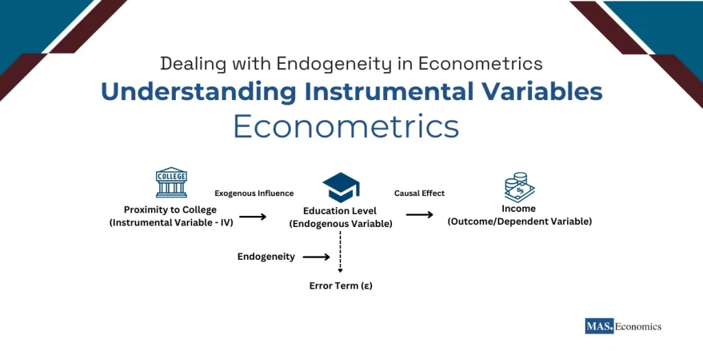
   Example: In the context of estimating the effect of education (\( X \)) on income (\( Y \)), proximity to colleges (\( Z \)) is often used as an instrument. Living closer to a college increases the likelihood of attending college, thereby making \( Z \) a relevant predictor of \( X \).
2. Exogeneity:
   The instrument must not be correlated with the error term (\( \epsilon \)) in the regression model. This ensures that the instrument affects the dependent variable (\( Y \)) only through the endogenous variable (\( X \)) and not through any unobserved factors.
   Example: Continuing with the education example, proximity to colleges (\( Z \)) satisfies the exogeneity condition if we assume that geographic location has no direct effect on income (\( Y \)) apart from its impact on education (\( X \)).

Together, these conditions guarantee that the instrument can break the correlation between \( X \) and the error term (\( \epsilon \)), solving the problem of endogeneity.

How Instrumental Variables Work in Practice

The implementation of IVs typically involves a two-step estimation process known as Two-Stage Least Squares (2SLS). Let’s break it down in simple terms:

First Stage

In the first step, we use the instrument (\( Z \)) to predict the endogenous variable (\( X \)). This involves regressing \( X \) on \( Z \):

Here, \( \hat{X}_i \), the predicted values of \( X \), represent the variation in \( X \) that is driven purely by the instrument (\( Z \)).

Think of this step as “filtering out” the problematic variation in \( X \). Instead of using the observed \( X \), which may be correlated with the error term (\( \epsilon \)), we use \( \hat{X}_i \), which is uncorrelated with \( \epsilon \).

Second Stage

In the second step, we replace \( X \) with \( \hat{X} \) in the original regression model and estimate the relationship between \( Y \) and \( \hat{X} \):

Because \( \hat{X}_i \) is uncorrelated with \( \epsilon \), this regression produces consistent estimates of \( \beta_1 \), the causal effect of \( X \) on \( Y \).

Practical Example: Education and Income

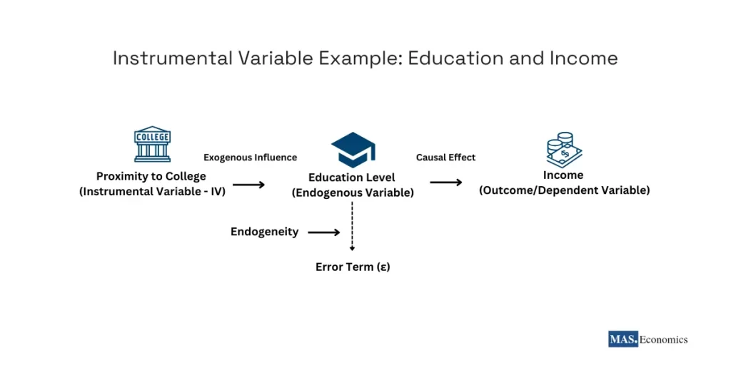
To demonstrate how IVs work, consider the relationship between education level (endogenous variable) and income (outcome variable). Researchers face endogeneity because unobserved factors, such as innate ability or family background, affect both education and income, biasing OLS estimates.

Proximity to College as an Instrument

To solve this, researchers use proximity to colleges as an instrumental variable:

• Relevance: Living close to a college increases the likelihood of pursuing higher education.

• Exogeneity: Proximity to college has no direct effect on income except through its influence on education.

Step-by-Step Implementation:

1. First Stage: Use proximity to college (\( Z \)) to predict education level (\( \hat{X} \)).
   \[ \text{Education Level} = \pi_0 + \pi_1 (\text{Proximity to College}) + \nu \]

2. Second Stage: Use the predicted education level (\( \hat{X} \)) to estimate its effect on income:
   \[ \text{Income} = \beta_0 + \beta_1 (\text{Education Level}) + u \]

This approach removes the endogeneity bias, allowing researchers to measure the causal effect of education on income accurately.

The Hausman Test: Validating the Use of IVs

The Hausman test is a widely used diagnostic tool in econometrics that helps determine whether an explanatory variable is endogenous and whether instrumental variables are necessary. It provides a formal way to compare the results of OLS and IV estimations.

Purpose of the Hausman Test

The Hausman test essentially asks: “Do the OLS and IV estimates differ significantly?” If they do, it indicates that the explanatory variable is endogenous, and the OLS estimates are biased. In such cases, IV methods are justified.

On the other hand, if the OLS and IV estimates are similar, it suggests that endogeneity is not a serious problem, and OLS can be used without introducing the complexity of IV methods.

Steps in the Hausman Test

1. OLS Estimation:
   First, estimate the model using OLS to obtain \( \hat{\beta}_{OLS} \), the coefficient estimates from the standard regression.
2. IV Estimation:
   Next, estimate the model using IV methods (e.g., 2SLS) to obtain \( \hat{\beta}_{IV} \), the coefficient estimates accounting for endogeneity.
3. Hypothesis Testing:
   Test the null hypothesis:
   \[ H_0 : \hat{\beta}_{OLS} = \hat{\beta}_{IV} \]
   • If the null hypothesis is rejected, it indicates that the OLS estimates are biased due to endogeneity, validating the use of IV methods.
   • If the null hypothesis is not rejected, it suggests that endogeneity is not a concern, and OLS estimates are reliable.

When to Use the Hausman Test

The Hausman test is particularly useful in cases where the presence of endogeneity is uncertain. For example, in studying the relationship between healthcare access and health outcomes, researchers might use policy changes as instruments. The Hausman test can confirm whether OLS estimates are biased by endogeneity, justifying the use of IVs.

Mathematical Framework for the Hausman Test

The Hausman test evaluates the difference between the OLS and IV estimates, taking into account their variances. Here’s how it works mathematically:

1. Define the difference between the OLS and IV estimates:
   \[ d = \hat{\beta}_{OLS} – \hat{\beta}_{IV} \]

2. Calculate the variance of the difference:
   \[ \text{Var}(d) = \text{Var}(\hat{\beta}_{OLS}) – \text{Var}(\hat{\beta}_{IV}) \]

3. Construct the test statistic:
   \[ H = d’ \left[ \text{Var}(d) \right]^{-1} d \]
   Under the null hypothesis (\( H_0 \)), this test statistic follows a chi-square distribution with degrees of freedom equal to the number of endogenous variables.


4. Decision Rule:
   • If \( H \) exceeds the critical value from the chi-square table, reject \( H_0 \) and conclude that the OLS estimates are biased.
   • Otherwise, fail to reject \( H_0 \), indicating that OLS estimates are consistent and IVs are unnecessary.

Intuitive Explanation

Think of the Hausman test as a “comparison tool.” If OLS and IV estimates are close to each other, it implies that the explanatory variable is not causing significant bias. But if they are far apart, it’s a red flag that endogeneity is present, and IVs are needed to correct the bias.

Example Application

Consider a study on the impact of advertising on sales. If researchers suspect that reverse causality exists (i.e., higher sales might lead to more advertising), they could use historical advertising budgets as an instrument. The Hausman test can confirm whether the suspected endogeneity is real and whether IV methods should replace OLS.

Challenges and Applications of IVs

While instrumental variables (IVs) are a powerful tool for addressing endogeneity, they are not without challenges. Applying IV methods requires careful consideration to ensure their validity and reliability.

Challenges in Using IVs

Finding Valid Instruments

Identifying instruments that satisfy both relevance and exogeneity is often challenging. A weak or poorly chosen instrument can introduce new biases instead of resolving existing ones.

Weak Instruments

An instrument is considered weak if it has a low correlation with the endogenous variable. Weak instruments reduce the precision of IV estimates and may lead to biased results even when exogeneity holds. Researchers often use statistical tests, such as the Cragg-Donald test, to evaluate instrument strength.

Generalizability

IV estimates often represent the local average treatment effect (LATE), which applies to the specific population influenced by the instrument. This limitation may reduce the generalizability of findings to the broader population.

Applications of IVs

Instrumental variables have been widely used in various fields:

Public Policy

Random assignment in social programs provides a natural experiment for evaluating policy effectiveness, with IVs helping isolate causal effects.

Economics

IVs are often used to estimate the causal effects of education, labor policies, and taxation. For example, proximity to colleges serves as an instrument in studies on the returns to education.

Healthcare

Policy changes, such as Medicaid expansions, are frequently used as instruments to study the impact of insurance access on health outcomes.

Conclusion

The instrumental variables (IV) approach offers an effective solution to address endogeneity in econometrics. By ensuring relevance and exogeneity, IVs enable researchers to obtain consistent and unbiased estimates of causal relationships, even when standard methods fail due to bias. The Hausman test further supports the validity of IVs by determining their necessity and confirming their appropriateness in addressing endogeneity issues.

A solid grasp of IV methods and their validation tools improves the reliability of econometric analyses, ensuring more accurate and meaningful insights in economic research.

FAQs:

What is endogeneity in econometrics?

Endogeneity occurs when one or more explanatory variables in a regression model are correlated with the error term, leading to biased and inconsistent estimates. It violates the core assumption of ordinary least squares (OLS) regression that independent variables should be exogenous.

What causes endogeneity?

Endogeneity arises due to factors like omitted variable bias, measurement error, simultaneity (reverse causality), or selection bias. These factors create correlations between explanatory variables and the error term, compromising the reliability of regression estimates.

How do instrumental variables solve endogeneity?

Instrumental variables (IVs) address endogeneity by isolating the exogenous variation in an independent variable. A valid IV must be strongly correlated with the endogenous variable (relevance) and uncorrelated with the error term (exogeneity). This ensures unbiased and consistent estimates.

What is the two-stage least squares (2SLS) method?

Two-stage least squares (2SLS) is a technique for implementing IVs. In the first stage, the endogenous variable is regressed on the instrument to obtain predicted values. In the second stage, these predicted values are used in place of the endogenous variable in the main regression to estimate the causal relationship.

What is the Hausman test, and why is it used?

The Hausman test compares OLS and IV estimates to determine whether endogeneity is a problem. If the OLS and IV estimates differ significantly, it indicates endogeneity, justifying the use of IVs. If not, OLS estimates can be considered reliable.

What challenges arise with instrumental variables?

Finding valid instruments is challenging, as they must meet both relevance and exogeneity conditions. Weak instruments can lead to imprecise estimates, and IV results may reflect a local average treatment effect (LATE), which may not generalize to the entire population.

Thanks for reading! Share this with friends and spread the knowledge if you found it helpful.
Happy learning with MASEconomics