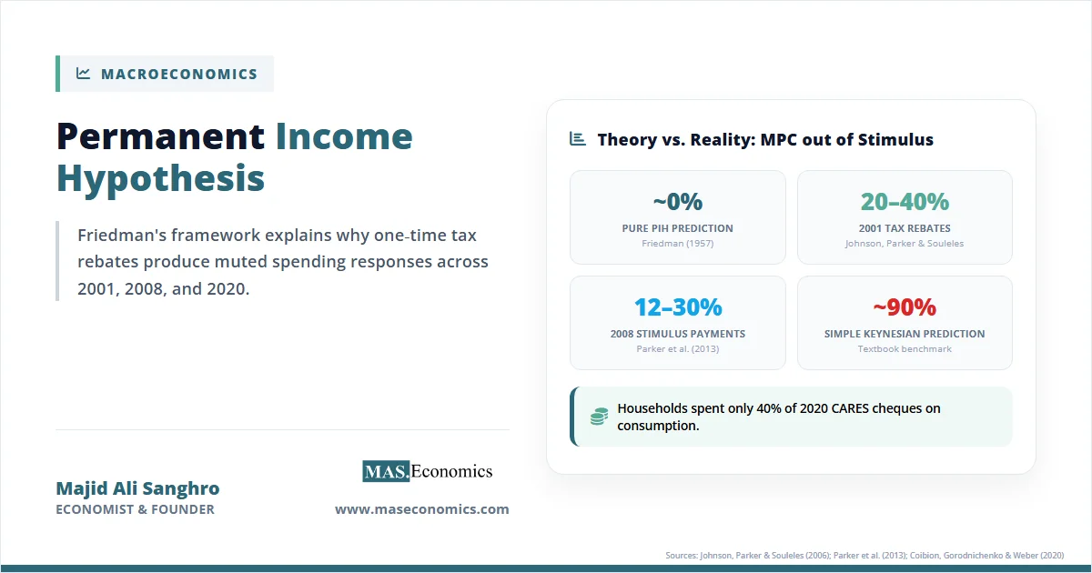
In May 2008, the US Treasury mailed roughly $100 billion in stimulus cheques to American households, hoping to jolt a faltering economy back into spending. By the end of that quarter, households had spent only between 12 and 30 percent of those payments on non-durable goods. The simple Keynesian textbook said the marginal propensity to consume should be close to 0.9. The data said it was closer to 0.2. The permanent income hypothesis, developed by Milton Friedman in 1957, predicts exactly this gap, and it has reshaped how economists think about fiscal policy ever since.
The puzzle is not academic. The 2001 rebates, the 2008 stimulus payments, and the 2020 CARES Act cheques all produced spending responses far below what one-shot Keynesian multipliers would predict. Friedman’s framework explains why: households do not consume out of the cheque in their hand. They consume out of the stream of income they expect to receive over a lifetime. A one-time payment barely shifts that stream, and so it barely shifts spending.
The Idea Friedman Introduced
Friedman’s 1957 book, A Theory of the Consumption Function, split household income into two pieces. Permanent income is the long-run, expected average a household believes it will earn. Transitory income is the deviation from that average in any given period, whether positive (a bonus, a tax refund, a lottery win) or negative (a temporary layoff, a one-off medical expense). Consumption, Friedman argued, depends almost entirely on permanent income. Transitory shocks are smoothed away through saving and borrowing.
The implication is direct. If a household earns $60,000 in a normal year and unexpectedly receives a $1,200 cheque, the household does not believe its lifetime earnings have just risen by $1,200. It treats the cheque as a one-off windfall. Spreading $1,200 over a remaining working life of, say, thirty years adds only about $40 a year to permanent income. The marginal propensity to consume out of that transitory dollar is correspondingly small.
This contrasts sharply with the simple Keynesian consumption function, where current disposable income drives spending almost mechanically. In Keynes’s framework, every extra dollar of disposable income produces a roughly proportional increase in consumption, with multipliers of two or three not uncommon in textbook calculations. Friedman’s framework predicts the opposite: anticipated and one-off changes in current income should produce muted spending responses, because rational households have already factored them into their lifetime plan.
How Households Smooth Income
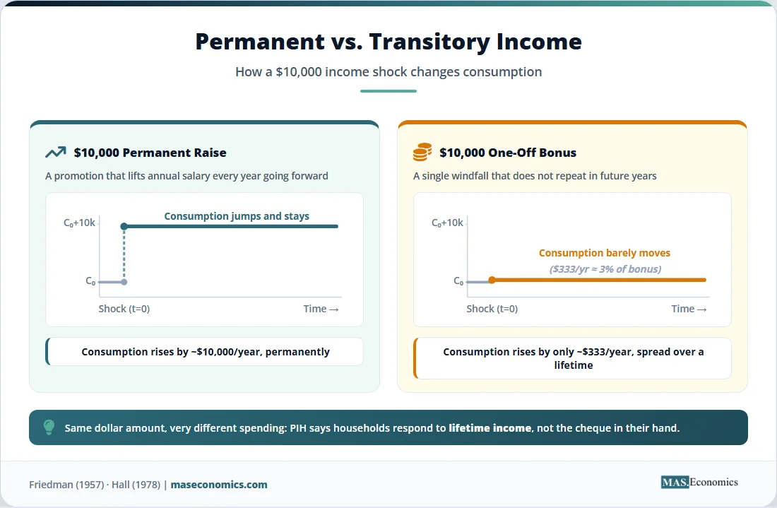
Consumption smoothing is the practical engine of the hypothesis. Imagine a worker whose income jumps by $10,000 because of a one-year contract. Under simple Keynesian rules, spending would rise sharply that year and fall back the next. Under Friedman’s framework, the household saves most of the bonus, draws on those savings in the future, and keeps consumption nearly flat across years.
The same logic runs in reverse. A worker temporarily laid off for three months does not slash spending in proportion to the income loss. The household borrows, draws down savings, or postpones large purchases. As long as the lifetime earnings path is largely intact, current consumption stays close to its long-run level. This is why aggregate consumption is much smoother than aggregate income across the business cycle, a stylised fact that simple Keynesian models struggle to explain.
Robert Hall extended Friedman’s framework in 1978 by adding rational expectations. If households use all available information to forecast lifetime resources, then changes in consumption should be unpredictable. Only genuine news, information that revises permanent income, should move spending. Anything already anticipated, including a tax cut announced months in advance, should already be embedded in current consumption. Hall’s “random walk” formulation turned the permanent income hypothesis into a sharp, testable prediction.
This rational-expectations layer matters for policy. A pre-announced tax rebate, under Hall’s logic, should produce no spending bump at the moment cheques arrive, because households updated their plans the day the policy was announced. Only the surprise component of fiscal policy can move consumption. That is a far cry from the headline-grabbing stimulus calculations many policymakers still rely on.
The Equations Behind the Theory
The simplest form of the permanent income hypothesis writes consumption as a constant fraction of permanent income:
where \( C_t \) is consumption in period \( t \), \( Y_t^p \) is permanent income, and \( k \) is the propensity to consume out of permanent income (close to one for long-lived households). Total measured income is the sum of permanent and transitory components:
Because transitory income \( Y_t^T \) does not enter the consumption equation, the marginal propensity to consume out of a temporary windfall is approximately zero in the pure form of the model. Of course, real households do spend some of their windfalls, which is why the empirical literature treats this as a benchmark rather than a literal description.
A more modern way to state the same idea uses the consumption Euler equation derived from a two-period optimisation problem. A household maximises lifetime utility:
subject to the lifetime budget constraint:
where \( \delta \) is the rate of time preference, \( r \) is the interest rate, and \( A_0 \) is initial wealth. The first-order condition is the consumption Euler equation:
When \( r = \delta \), the household equalises expected marginal utility across periods. With quadratic utility, this collapses to Hall’s prediction that consumption follows a random walk: \( E_1[C_2] = C_1 \). Forecastable income changes, including pre-announced stimulus payments, should not change \( C_1 \), because they were already incorporated into the household’s plan.
| Symbol | Meaning | Role in the Model |
|---|---|---|
| \( C_t \) | Consumption in period \( t \) | The variable households choose |
| \( Y_t^p \) | Permanent income | Long-run expected income |
| \( Y_t^T \) | Transitory income | Temporary deviation from permanent |
| \( k \) | Propensity out of permanent income | Close to 1 for infinite-lived households |
| \( \delta \) | Rate of time preference | How much households discount the future |
| \( r \) | Real interest rate | Return on saving and cost of borrowing |
| \( A_0 \) | Initial wealth | Starting financial assets |
| \( E_t[\cdot] \) | Expectation given period-\( t \) information | Captures rational forecasting |
 | ||
Table 1. Variables in the Permanent Income Hypothesis: Notation and economic meaning.
Consumption Smoothing in the Data
The cleanest illustration comes from comparing how households react to permanent versus transitory income changes. A worker who lands a permanent promotion with a 20 percent salary increase typically raises consumption by something close to 20 percent. A worker who receives an end-of-year bonus equal to 20 percent of their annual salary, knowing it is a one-off, raises consumption by far less. This is exactly what Friedman’s hypothesis predicts.
Aggregate data tell a similar story. US personal consumption expenditures move much more smoothly than disposable personal income across the business cycle. During the 2020 lockdown, disposable income spiked because of stimulus payments and unemployment insurance top-ups, while consumer spending fell sharply because of restricted activity. The gap appeared as a record surge in the personal saving rate, briefly reaching 32 percent in April 2020, according to Federal Reserve Economic Data. Households treated the unusual income spike as transitory and saved most of it, just as Friedman would have predicted.
The smoothing logic also explains a stylised fact that puzzled early Keynesian economists. In simple Keynesian models, a temporary income drop of, say, 10 percent should produce a near-proportional consumption drop, deepening the recession through the multiplier. In the US recession data, that proportionality breaks down. Consumption typically falls by far less than income during downturns because households expect the slump to end and draw on savings, credit, and home equity to keep spending closer to its long-run path. The same logic flips during expansions: when household income surges in a boom, much of it is saved rather than spent on a one-for-one basis. This asymmetry between income volatility and consumption stability is one of the most robust findings in modern macroeconomics, and Friedman’s framework was the first to provide a coherent theoretical explanation for it.
What the Theory Assumes
The pure form of the permanent income hypothesis rests on three demanding assumptions. The first is rationality and forward-looking behaviour. Households are assumed to forecast lifetime income accurately, update those forecasts when new information arrives, and choose consumption to maximise expected lifetime utility. Real households use rules of thumb, mental accounts, and shortcuts that depart from this ideal.
The second assumption is access to financial markets. To smooth consumption against transitory shocks, households need to save freely when income is high and borrow freely when income is low. Friedman’s model implicitly assumes capital markets work well enough to make this possible. When they do not, the model’s predictions break down sharply.
The third assumption is the absence of binding liquidity constraints. A household that wants to borrow against future earnings but cannot, because banks will not lend to it, behaves very differently from an unconstrained one. For such a household, consumption tracks current income closely, because there is no other option. The marginal propensity to consume out of a stimulus cheque, in this case, can be very high.
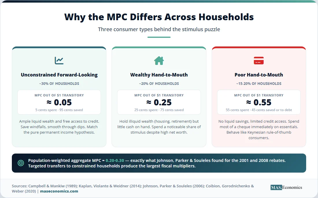
These limitations matter for policy. Campbell and Mankiw, in their 1989 paper, formalised the idea that the population is split between forward-looking, permanent-income consumers and “rule-of-thumb” consumers who simply spend their current income. Their estimates suggested that roughly half of US aggregate income flows to households that behave like rule-of-thumb consumers. This hybrid model fits the data better than either pure Keynesian or pure permanent income models alone, and it is closer to what modern macro models assume.
Testing the Hypothesis
Hall’s 1978 paper was the first formal test. He examined US time-series data and found that, to a first approximation, lagged income did not help predict changes in consumption once lagged consumption was included. The random walk prediction held reasonably well in aggregate data, although stock prices did predict consumption changes, hinting that the theory was incomplete.
The most powerful tests came from natural experiments. The 2001 US tax rebates, sent out between July and September of that year, were timed by the second-to-last digit of the recipient’s Social Security number, which is effectively random. Johnson, Parker, and Souleles (2006) exploited this randomisation in the Consumer Expenditure Survey. They found that households spent 20 to 40 percent of their rebates on non-durable goods in the three-month window of receipt, with another third in the following quarter. This is far more than the pure permanent income hypothesis predicts (essentially zero) but far less than the simple Keynesian prediction.
The 2008 stimulus payments produced a similar pattern. Parker, Souleles, Johnson, and McClelland (2013) found that households spent 12 to 30 percent of payments on non-durables in the receipt quarter, with sizeable additional spending on durable goods (mainly vehicles), bringing the total response to between 50 and 90 percent over a longer window. The response was concentrated among older, lower-income, and home-owning households, which is consistent with the binding-liquidity-constraint story rather than the pure permanent income view.
The 2020 CARES Act cheques tell the same broad story. Coibion, Gorodnichenko, and Weber (2020), using a survey of 12,000 Americans, found that respondents reported spending only about 40 percent of their stimulus payments. Around 30 percent was saved, and another 30 percent went to debt repayment. About 40 percent of respondents reported not spending any of their cheque, and only around 30 percent reported spending the entire amount. The lower spending rates were concentrated among those without binding liquidity constraints, exactly as Friedman’s framework predicts.
Figure 1. Marginal propensity to consume out of stimulus payments by episode (non-durable spending, three-month window). Sources: Johnson, Parker, and Souleles (2006); Parker et al. (2013); Coibion, Gorodnichenko, and Weber (2020).
Three patterns emerge across these studies. First, observed marginal propensities to consume sit between the pure permanent income prediction and the simple Keynesian prediction. Second, the response is consistently larger for liquidity-constrained, low-wealth, and low-income households. Third, durable goods spending often dominates non-durable spending in the response, which suggests that stimulus cheques pull forward planned purchases rather than create entirely new ones.
Why It Still Shapes Policy
The permanent income hypothesis still shapes how serious fiscal policy is designed, even when its pure form is rejected. Three implications dominate the modern policy debate.
First, the framework explains why broad, untargeted stimuli tend to underperform expectations. When governments mail cheques to everyone, including high-income households with ample savings, much of the money is saved or used to repay debt rather than spent. The aggregate fiscal multiplier ends up well below the simple Keynesian benchmark. This is a key reason why fiscal multiplier estimates have shifted downward in academic and policy work since the 2000s. The 2020 CARES Act, despite its $2 trillion price tag, produced muted near-term consumption growth precisely because much of the money landed in households for whom the cheques were a transitory windfall.
Second, the empirical evidence on liquidity-constrained households has driven a clear shift towards targeted transfers. If the goal is to boost aggregate demand, and if only liquidity-constrained households spend most of a cheque, then sending the cheques to those households alone should generate more spending per dollar of public money. Recent US Earned Income Tax Credit expansions, the 2021 expanded Child Tax Credit, and various state-level programmes have explicitly leaned on this logic. The empirical literature now reports much higher MPCs for low-income, low-liquidity households, often above 0.5, while high-income households show MPCs near zero.
Third, the hypothesis is central to the universal basic income debate. Supporters argue that permanent, unconditional transfers would shift recipients’ permanent income upward and produce sustained spending and labour-supply effects. Critics, drawing on the same framework, argue that financing such a permanent transfer through higher permanent taxes would leave aggregate permanent income unchanged, with offsetting effects on saving and labour supply. The debate over permanent versus transitory financing of basic income programmes is, in essence, an applied permanent income hypothesis question.
The framework also informs the timing of tax cuts. A pre-announced, temporary cut, under Hall’s logic, has its main effect at the moment of announcement, not at the moment of implementation. A permanent cut affects spending sustainably; a temporary one affects it only modestly and briefly. This logic shaped much of the analysis around the 2017 US Tax Cuts and Jobs Act, where economists carefully distinguished between provisions set to expire and those made permanent.
Finally, the permanent income hypothesis is a quiet pillar of modern debt sustainability analysis. If households are forward-looking and care about lifetime resources, then current government deficits financed by future taxes may produce smaller spending boosts than naive multiplier calculations suggest, an effect known as Ricardian equivalence. Although strict Ricardian equivalence is rarely supported in the data, the partial response of households to anticipated future taxes is a direct descendant of Friedman’s framework.
The hypothesis also reshaped the macroeconomic consumption function itself. The naive linear function used in early Keynesian models, where consumption is a fixed share of current disposable income, no longer survives in serious macro work. Modern dynamic stochastic general equilibrium models embed forward-looking consumers, and even hybrid New Keynesian frameworks like the Keynesian cross tradition now incorporate a fraction of liquidity-constrained households. The architecture of fiscal policy analysis rests on this hybrid view.
One concrete legacy of the framework is visible in how central banks now read the data. When the personal saving rate spikes during a stimulus episode, modern policy economists no longer treat the cheques as failed Keynesian instruments. They read the saving rate as evidence that the average household correctly identified the transfer as transitory. The relevant policy questions shift towards whether the stimulus reached liquidity-constrained households, whether durable goods purchases were merely pulled forward from later quarters, and whether the saved share might re-enter spending later when conditions normalise. This last question, sometimes called the “delayed multiplier”, has become important for analysing the post-2020 inflation surge: the unusual buildup of household savings during 2020 and 2021 likely contributed to the strong demand pressure that emerged once the economy reopened, even though the cheques themselves produced muted contemporaneous spending. Friedman’s framework, in other words, helps explain not just why stimulus disappoints in the moment, but also why its effects can show up much later in surprising places.
MASEconomics Explains
4 economic concepts behind the permanent income hypothesis
Conclusion
The permanent income hypothesis remains the most influential single idea in the modern theory of consumption. Friedman’s claim that households consume out of expected lifetime income, not current income, explains the muted response to one-off stimulus cheques across the 2001, 2008, and 2020 episodes. Empirical estimates put the marginal propensity to consume out of these payments at roughly 0.12 to 0.40 in the receipt quarter, well above the pure model’s near-zero prediction but far below the simple Keynesian benchmark of 0.9. The gap is largely explained by liquidity-constrained households, who behave more like Keynesian rule-of-thumb consumers, and unconstrained households, who behave more like Friedman’s forward-looking optimisers. The shift towards targeted transfers, the design of permanent versus temporary tax changes, and the analysis of universal basic income proposals all rest on this two-type consumer framework. Friedman’s hypothesis no longer survives in pure form, but the questions it forced economists to ask, about how anticipated, transitory, and permanent income changes feed into spending, remain the core of fiscal policy analysis today.
Did you find this article helpful? Share it with someone who loves economics. And remember, at MASEconomics, we make complex ideas simple.