What happens when a government spends one rupee during a recession? Does that rupee simply go into someone’s pocket and vanish, or does it ripple through the economy, creating many more rupees of income?
For most of the 20th century, economists believed the answer was the former. The classical view held that any increase in government spending would simply “crowd out” private spending, leaving total output unchanged. Then, in 1936, a British economist named John Maynard Keynes published a book that turned this idea on its head. He argued that government spending could actually increase total output by much more than the initial amount, through a mechanism he called the multiplier.
Why the Great Depression Seemed Impossible
To understand why Keynes’s idea was so radical, we need to look at the economics of the 1920s.
The classical economists, Adam Smith, David Ricardo, and their successors, had built a beautiful theory. They argued that markets, left to themselves, would always adjust to ensure full employment. If there were a temporary slump, wages and prices would fall, making goods cheaper and encouraging spending, and the economy would quickly bounce back. This was encapsulated in Say’s Law: “Supply creates its own demand.” In other words, producing goods generates enough income to buy them all. Mass unemployment, in this view, was a temporary aberration, not something that could persist.
When the Great Depression struck in the 1930s, unemployment soared to 25% in the United States and remained high for years. Classical economists were baffled. Wages fell, yet unemployment did not go away. Something was fundamentally wrong with the theory.
Keynes set out to find what was missing. His answer: aggregate demand. He argued that total spending in the economy, the sum of consumption, investment, and government spending, could fall short of what was needed to keep everyone employed. And when that happened, there was no automatic mechanism to restore full employment.
The Man Behind the Revolution
John Maynard Keynes (1883–1946) was no ordinary economist. He was a brilliant mathematician, a successful investor, a member of the Bloomsbury Group of artists and writers, and a key figure in British government during both world wars. His earlier work had already made him famous, but it was The General Theory of Employment, Interest and Money (1936) that would change economics forever.
Keynes wrote the book during the depths of the Depression, with millions unemployed. He was not just theorizing; he was trying to save capitalism from itself. As he famously put it, “Practical men, who believe themselves to be quite exempt from any intellectual influences, are usually the slaves of some defunct economist.” He wanted to replace the old doctrines with ones that could guide policymakers to restore prosperity.
The General Theory was dense and difficult, but its central idea, that aggregate demand determines output, could be captured in a simple diagram: the Keynesian cross.
The Core Idea: Aggregate Demand
Keynes’s key insight was that in the short run, output is determined by planned spending, what households, businesses, and the government intend to buy. If planned spending is less than what firms are producing, inventories pile up, and firms cut production. If planned spending exceeds production, inventories fall, and firms increase production. Output adjusts until it equals planned spending.
In a closed economy with no government, planned spending is simply consumption \(C\). But consumption itself depends on income. Keynes proposed a “psychological law”: as income rises, consumption rises, but by less than the increase in income. The fraction of extra income that goes to consumption is the marginal propensity to consume (MPC), a number between 0 and 1.
So we have:
\text{Planned spending} = C = \bar{C} + MPC \times Y
$$
where \(\bar{C}\) is autonomous consumption, what people would spend even if income were zero.
In equilibrium, output \(Y\) must equal planned spending:
Y = \bar{C} + MPC \times Y
$$
Solving for \(Y\) gives:
Y = \frac{\bar{C}}{1 – MPC}
$$
This is the multiplier in its simplest form: an increase in autonomous spending (say, from a government stimulus) is multiplied by a factor \(\frac{1}{1 – MPC}\) to produce a larger increase in output.
The Multiplier in Action: A MASEconomics Example
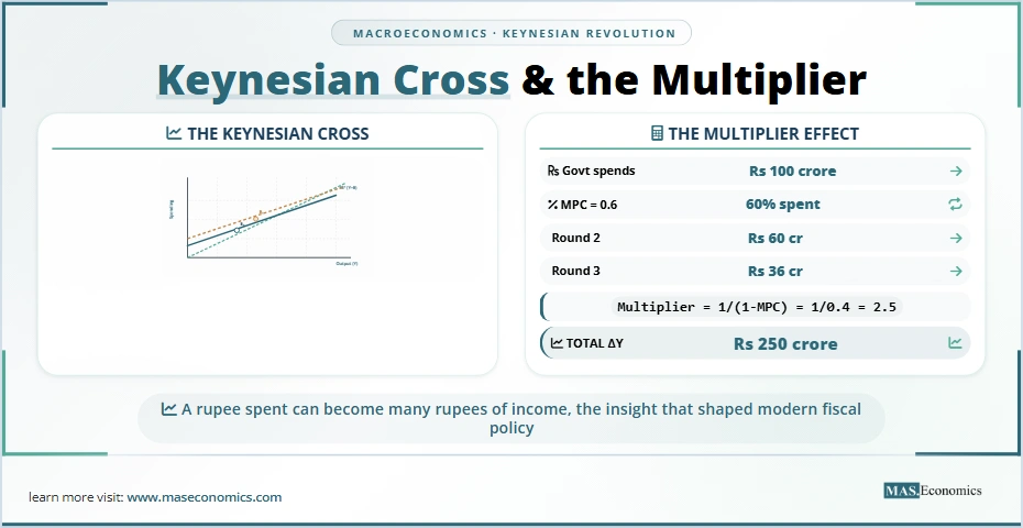
Consider Pakistan during a recession. Suppose the government decides to spend Rs 100 crore on a new infrastructure project. This Rs 100 crore becomes income for the workers and suppliers. They, in turn, spend a portion of it. Let us assume the marginal propensity to consume is 0.6, meaning that for every additional rupee of income, people spend 60 paise and save 40 paise.
The initial Rs 100 crore becomes income for others, who spend 60% of it: Rs 60 crore. That Rs 60 crore becomes income for yet others, who spend 60% of it: Rs 36 crore. And so on. The total increase in income is:
100 + 60 + 36 + 21.6 + \cdots = \frac{100}{1 – 0.6} = 250 \text{ crore}
$$
So the multiplier is 2.5. A Rs 100 crore government project raises total income by Rs 250 crore.
Keynes called this the investment multiplier. In his 1931 article, Richard Kahn had introduced the concept of the employment multiplier, but Keynes gave it its modern form.
The Keynesian Cross Diagram
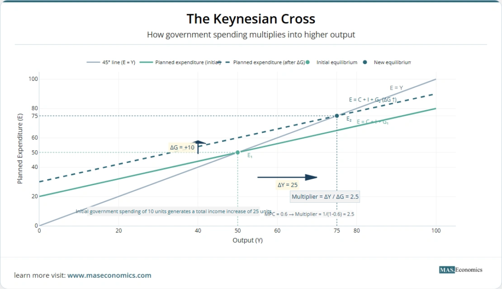
The simplest way to visualize this is with a diagram. On the horizontal axis, we plot total output \(Y\). On the vertical axis, we plot planned spending \(E\). The 45‑degree line represents all points where output equals planned spending (\(E = Y\)).
The consumption function is a line with slope \(MPC\) and intercept \(\bar{C}\). Add government spending \(G\) and investment \(I\) to get total planned spending
E = \bar{C} + I + G + MPC \times Y
$$
The equilibrium output is where this line crosses the 45‑degree line.
If the government increases spending, the line shifts up by \(\Delta G\). The new equilibrium is at a higher \(Y\), and the increase in \(Y\) is larger than \(\Delta G\) because of the multiplier.
This simple diagram became the centerpiece of introductory macroeconomics. It showed, in one picture, why fiscal policy could work.
The Paradox of Thrift
One of Keynes’s most counterintuitive insights was the paradox of thrift. In classical economics, saving was seen as virtuous; it provided funds for investment. But Keynes showed that if everyone tries to save more, total spending falls, output falls, and in the end, total saving may not increase at all.
Suppose households decide to increase their savings rate. That means they consume less, shifting the planned spending line down. Output falls, and with lower income, the amount saved (which is a fraction of income) may actually fall. The attempt to save more backfires.
This paradox illustrates the core of Keynesian thinking: what is prudent for an individual may be disastrous for the economy as a whole.
Extensions and Refinements
The Accelerator and Business Cycles
The simple Keynesian cross assumed investment was fixed. In reality, investment depends on output. When the economy grows, firms invest to expand capacity. This insight led to the accelerator principle: investment is proportional to the change in output. When combined with the multiplier, it can generate cycles. Paul Samuelson’s 1939 paper showed how the multiplier-accelerator model could produce business cycles with booms and busts.
The IS‑LM Framework
John Hicks, in his 1937 paper “Mr. Keynes and the Classics,” provided a way to integrate Keynes’s theory with monetary policy. The IS curve represents equilibrium in the goods market (the Keynesian cross) for different interest rates. The LM curve represents equilibrium in the money market. Together, they determine both output and the interest rate. This became the workhorse model for macroeconomics for decades.
The Multiplier with Taxes
If the government finances spending with taxes, the multiplier changes. A balanced‑budget multiplier (where spending is matched by taxes) is exactly 1, a result derived by Trygve Haavelmo in 1945. If taxes are lump‑sum, the multiplier is smaller because higher taxes reduce consumption. If taxes are progressive, the distributional effects matter, as modern research shows.
Heterogeneous Marginal Propensities to Consume
For many years, economists assumed that the MPC was a stable number, around 0.6 to 0.7. But recent research, using microdata, has shown that the MPC varies enormously across households.
Using lottery winnings in Norway, Fagereng, Holm, and Natvik (2021) found that the average MPC is about 0.51 in the year of the win, but it varies widely. Some households spend almost the entire windfall; others save most of it. The MPC is much higher for households with low wealth and low income.
This matters for fiscal policy. If a stimulus check is given to poor households, they spend a large fraction, generating a big multiplier. If it is given to wealthy households, they save more, and the multiplier is smaller.
The 2024 paper by Auclert, Rognlie, and Straub develops an intertemporal Keynesian cross that incorporates these heterogeneous MPCs. They show that the response to fiscal policy depends on the entire time‑path of income and on the distribution of MPCs across households. In their model, deficit‑financed spending can have a multiplier greater than one, especially if the MPC is high for many households.
This modern work brings Keynes’s original insight full circle: the multiplier is not just a theoretical curiosity; it is a measurable, policy‑relevant number that depends on the structure of the economy and the design of the stimulus.
Critiques and Limitations
No theory is perfect, and the Keynesian cross has been criticized on many grounds.
Ricardian equivalence – Some economists argue that households anticipate future taxes to pay for deficit spending and will save the extra income, leaving output unchanged.
Supply‑side effects – Higher government spending may crowd out private investment by raising interest rates.
Open economy – In a country like Pakistan, part of the stimulus may leak abroad through imports, reducing the domestic multiplier.
Liquidity traps – When interest rates are already zero, the multiplier can be larger, but monetary policy may be ineffective.
Microfoundations – Modern macroeconomics insists that models be based on optimizing behavior. The simple Keynesian cross has been replaced by New Keynesian models that include price stickiness, rational expectations, and heterogeneous agents.
Nevertheless, the basic intuition remains. When there is slack in the economy, government spending can increase output, and the multiplier can be substantial.
Does the Keynesian Cross Still Matter?
After all these critiques, you might wonder if the Keynesian cross is still relevant. The answer is a resounding yes. Here is why.
As a Pedagogical Tool
The Keynesian cross is the first model every economics student learns. It is simple, intuitive, and teaches the fundamental concept of aggregate demand. It provides the foundation for understanding more complex models.
As a Policy Framework
Fiscal stimulus debates still revolve around the multiplier. When governments consider infrastructure spending or tax cuts, they ask: how much will it boost output? The answer depends on the MPC, the degree of openness, and the state of the economy. The Keynesian cross provides the framework for asking these questions.
As a Historical Landmark
Keynes’s idea changed the world. Before him, governments believed they should balance budgets even in depressions. After him, deficit spending became an accepted tool to fight recessions. The Keynesian cross symbolizes that shift.
As a Bridge to Modern Research
Today’s heterogeneous‑agent models, like the intertemporal Keynesian cross, build directly on Keynes’s insight. They show that the multiplier is not a fixed number but depends on who receives the stimulus. This is exactly what policymakers need to know.
The Bottom Line
The Keynesian cross is a deceptively simple diagram with a profound implication: in a depressed economy, government spending can multiply into much larger increases in output. Keynes’s insight broke with centuries of classical thinking and laid the foundation for modern macroeconomics.
The multiplier is not a mechanical constant; it depends on how people respond to changes in income. Today, we know that the MPC varies widely across households, and that this matters for policy. But the core idea, that spending generates more spending, remains as relevant as ever.
So, the next time you hear a debate about fiscal stimulus, remember the Keynesian cross. Behind the arguments about debt and deficits lies a simple truth: in the right circumstances, a rupee spent by the government can do more than a rupee of private spending. It can set in motion a chain of spending that lifts the whole economy.
Did you find this article helpful? Share it with someone who loves economics. And remember, at MASEconomics, we make complex ideas simple.