Capital Mobility Open Economy: BP Curve and Policy

The same fiscal expansion can raise output sharply in one country and barely move it in another, even when both run identical policies, because the two differ in how freely capital crosses their borders. That single difference, the degree of capital mobility, decides whether a higher domestic interest rate pulls in a flood of foreign funds or barely a trickle. In open economy macroeconomics, capital mobility analysis turns on this question, because the responsiveness of cross-border flows to interest-rate differences is what gives the balance-of-payments curve its slope, and that slope determines which policy instruments work.

The concept is not a side detail in the open-economy model; it is the dial that sets the model’s behavior. The Mundell-Fleming model produces sharply different predictions about fiscal and monetary policy depending on whether capital is highly mobile, partly mobile, or immobile. Understanding capital mobility on its own terms, before it is plugged into a policy experiment, is what makes those predictions legible rather than arbitrary.

Measuring Capital Mobility

Capital mobility describes how strongly financial capital responds to differences in returns across countries. When an investor can move funds abroad cheaply, quickly, and without restriction, a small gap between the domestic interest rate and the world rate is enough to trigger large flows. When capital controls, transaction costs, currency risk, or thin financial markets stand in the way, even a wide interest-rate gap moves relatively little capital. Mobility is therefore a matter of degree, running from perfect at one extreme to zero at the other.

The cleanest way to express it is through the capital account, which records cross-border financial flows as a function of the interest-rate differential between the domestic rate \(i\) and the world rate \(i^{*}\).

Capital Account Flow

The parameter κ measures the degree of capital mobility. A large κ means capital responds strongly to a given interest-rate gap; κ near zero means it barely responds.

The parameter \(\kappa\) is the whole story in compact form. A large \(\kappa\) means a tiny interest-rate differential draws in large capital inflows, the signature of high mobility. A \(\kappa\) near zero means the capital account is nearly unresponsive, the signature of controls or deep frictions. As \(\kappa\) rises toward infinity, the model reaches the limiting case of perfect mobility, where the domestic interest rate cannot deviate from the world rate at all because any gap would trigger unbounded flows.

Mobility and the BP Curve Slope

The balance-of-payments curve, the BP schedule, traces the combinations of output and interest rate at which the external accounts are in equilibrium. Its slope is a direct expression of \(\kappa\). The relationship behind the curve sets the trade balance against the capital account, where the trade balance worsens as output rises and the capital account improves as the interest rate rises.

External Balance

Higher output Y raises imports and worsens net exports NX; a higher interest rate i raises the capital inflow. The slope of the BP curve in the Y-i plane is determined by κ.

The intuition runs through how much the interest rate must move to offset a rise in output. Suppose output increases, which raises imports and pushes the current account toward deficit. To keep the overall balance at zero, the capital account has to improve by an equal amount, which requires the interest rate to rise enough to attract the necessary inflow. If capital is highly mobile, a small rise in the interest rate brings in plenty of capital, so the BP curve is nearly flat. If capital is barely mobile, the interest rate has to rise a great deal to attract the same inflow, so the BP curve is steep. This logic builds on the accounting behind the balance of payments, where any current-account imbalance must be matched by an offsetting capital-account flow.

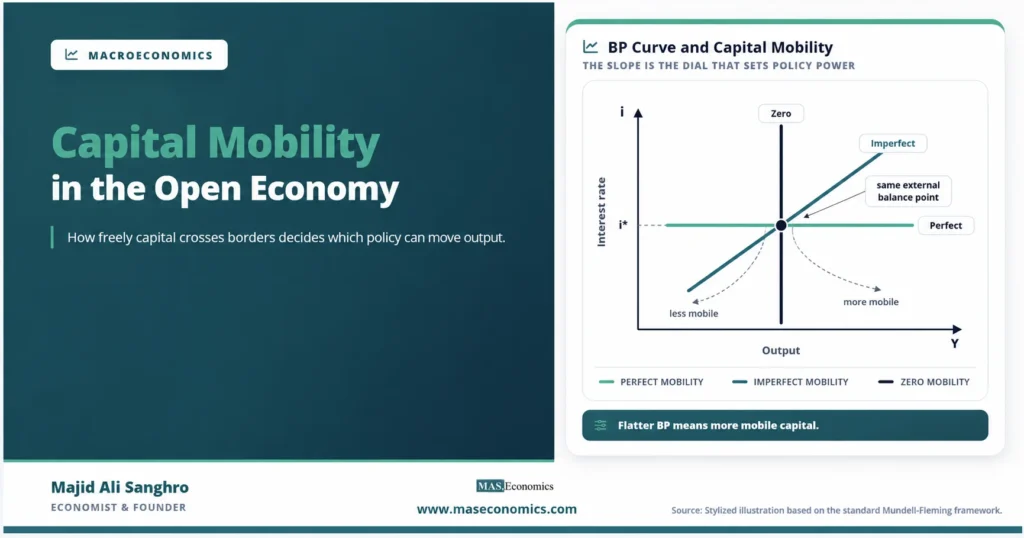
The diagram collapses the whole spectrum into one picture. The mint horizontal line is the perfect-mobility benchmark: the domestic interest rate is pinned at the world rate \(i^{*}\), because any deviation would trigger infinite flows. The navy vertical line is the zero-mobility case: the capital account cannot respond at all, so external balance depends entirely on the current account, and only one level of output is consistent with it. The teal upward-sloping line is the realistic intermediate case, where capital is mobile but not perfectly so, and the steepness of that line is exactly what \(\kappa\) controls. A flatter teal line means higher mobility; a steeper one means lower mobility.

Slope and Policy Effectiveness

The reason this matters is that the slope of the BP curve relative to the LM curve determines whether monetary and fiscal policy move output. The comparative-statics results that define open-economy macro all hinge on where the new internal equilibrium falls relative to the BP curve, and that in turn depends on how steep the BP curve is.

Table 1. Capital Mobility and Policy Effectiveness by Exchange-Rate Regime

Capital mobility	BP curve	Fixed rates: stronger tool	Floating rates: stronger tool
Perfect	Horizontal at i*	Fiscal policy fully effective	Monetary policy fully effective
High but imperfect	Flatter than LM	Fiscal policy strong	Monetary policy strong
Low but imperfect	Steeper than LM	Both partly effective	Both partly effective
Zero	Vertical	Monetary policy via reserves only	Exchange rate clears trade alone
Source: MASEconomics editorial synthesis of the Mundell-Fleming framework.

The clearest results sit at the perfect-mobility extreme. With a horizontal BP curve, fiscal policy is fully effective under fixed exchange rates because reserve flows expand the money supply to accommodate it, while monetary policy is powerless because any attempt to cut the interest rate is reversed by reserve losses. Under floating rates the conclusions flip: monetary policy is fully effective because depreciation reinforces it, while fiscal policy is neutralized by an offsetting appreciation. As mobility falls and the BP curve steepens, these sharp results soften, and both instruments retain partial effect. The degree of capital mobility is the knob that turns one regime’s policy world into the other’s.

Policy Trade-Off from Mobility

Capital mobility is not just a technical parameter; it is the source of a binding policy constraint. A country that opens its capital account and fixes its exchange rate discovers that it can no longer run an independent monetary policy, because defending the peg ties the money supply to reserve flows. A country that opens its capital account and floats regains monetary independence but gives up control of the exchange rate. The choice cannot be avoided once capital is mobile.

This is the open-economy trilemma. Of the three goals, a fixed exchange rate, free capital movement, and independent monetary policy, a country can hold at most two at once. High capital mobility is what makes the third goal unattainable alongside the other two, which is why the constraint did not bind under the capital controls of the Bretton Woods era and became sharp once financial markets integrated. The full structure of this constraint is the subject of the Mundell trilemma, which formalizes why the three goals are mutually incompatible.

Limitations of Simple Treatment

The linear capital-account relationship is a useful simplification, but it hides features that matter in practice. It treats capital flows as a smooth function of the interest-rate differential, when real flows also respond to expected exchange-rate changes, risk premia, and shifts in global financial conditions that have nothing to do with the domestic interest rate. A country can experience large inflows or outflows driven by sentiment abroad rather than by its own policy stance.

The model also assumes mobility is symmetric and stable, when episodes of sudden stops show that capital can flow in freely for years and then reverse in weeks. The parameter \(\kappa\) is best read as a description of normal-times responsiveness, not a guarantee that flows will behave the same way under stress. These limits do not undermine the core insight that the slope of the BP curve governs policy effectiveness; they qualify how confidently the static curve can be applied to a turbulent capital account.

Explains

Conclusion

The role of capital mobility open economy analysis is to set the slope of the balance-of-payments curve, and through that slope, to determine which policy instruments can move output. High mobility flattens the BP curve toward the horizontal benchmark, where the strongest Mundell-Fleming results hold; low mobility steepens it toward the vertical, where those results dissolve. The single parameter that measures how strongly capital responds to interest-rate differentials is what links the abstract diagram to the concrete behavior of fiscal and monetary policy.

The deeper point is that mobility is not neutral. Opening the capital account does not simply add a channel; it imposes a choice between a stable exchange rate and an independent monetary policy, because the two cannot coexist with free capital movement. This is why the degree of capital mobility sits at the center of open-economy macroeconomics rather than at its margin.

That centrality is also a reminder of the model’s limits. Treating mobility as a fixed parameter captures normal times well but misses the abrupt reversals that define financial crises. The BP curve describes where capital flows settle when conditions are calm; it does not predict when calm will give way to a sudden stop. Read with that caveat, capital mobility remains the most useful single lens for understanding why the same policy produces such different results across open economies.

Frequently Asked Questions

Thanks for reading! If you found this helpful, share it with friends and spread the knowledge. Happy learning with MASEconomics