Jacobian Matrix Economics: Comparative Statics and Stability

An exchange-rate model, a labor-market system, or a two-market general equilibrium model can change in several directions at once when one parameter shifts. Jacobian matrix economics gives economists a compact way to organize those simultaneous marginal effects and study comparative statics, local solvability, and stability.

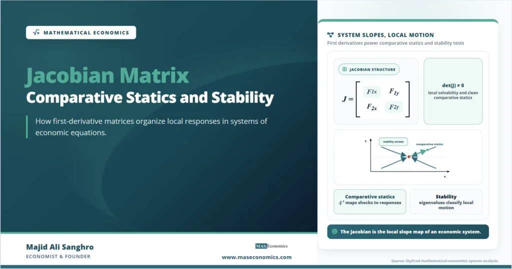
The Jacobian matrix is a matrix of first partial derivatives. It shows how a vector of functions changes when a vector of variables changes. In economics, that makes it useful wherever one equation is not enough: demand systems, equilibrium models, dynamic adjustment, input-output systems, and policy reaction functions.

The idea builds on differentiation and vectors and matrices. Differentiation gives marginal effects. Matrix notation organizes those effects into a system.

Systems need organized derivatives

Many economic models contain more than one equation. A single market may be described by supply and demand. A macroeconomic model may include goods-market equilibrium, money-market equilibrium, and a policy rule. A trade model may include several excess-demand equations linked by relative prices.

When one variable changes, the whole system can respond. A wage increase may affect labor supply, labor demand, output, prices, and income. A tax change may affect consumption, investment, government revenue, and equilibrium output. These responses are connected, not isolated.

A Jacobian matrix collects the derivatives of a system in one place. If a vector-valued function \(F(x)\) maps variables into equations, the Jacobian shows the local sensitivity of each equation to each variable.

Vector function

The Jacobian is the derivative matrix of this vector function. It is the multivariable equivalent of a slope, but for systems instead of one curve.

The Jacobian records marginal effects

For \(m\) functions and \(n\) variables, the Jacobian matrix is:

Jacobian matrix

Each row corresponds to one equation. Each column corresponds to one variable.

The entry in row \(i\), column \(j\), shows how equation \(F_i\) changes when variable \(x_j\) changes slightly, holding the other variables fixed. This is why the Jacobian is useful in comparative statics. It records the local structure of the whole model.

If \(m=n\), the Jacobian is square and has a determinant. That determinant is especially important. A nonzero determinant usually means the system can be locally solved for the endogenous variables. A zero determinant signals local degeneracy, redundancy, or failure of the usual comparative-static calculation.

Two equations show the structure

A simple two-equation model is enough to see the logic. Suppose an economy is described by two equilibrium conditions:

Two-equation system

The variables \(x\) and \(y\) are endogenous. The parameter \(a\) is exogenous.

The Jacobian with respect to the endogenous variables is:

Endogenous-variable Jacobian

The determinant is:

If \(\det(J)\neq 0\), the two equations are locally independent. Small parameter changes can be translated into small changes in \(x\) and \(y\). If \(\det(J)=0\), the model may not provide a unique local response.

Economically, a nonzero Jacobian determinant means the equilibrium conditions intersect cleanly near the point. A zero determinant means the system may be locally flat, tangent, redundant, or unstable in a way that prevents ordinary comparative statics.

Comparative statics uses the inverse

Comparative statics asks how equilibrium changes when a parameter changes. In the two-equation system, the total differential gives:

Total differential system

In matrix form:

If \(J\) is invertible, the equilibrium response is:

Comparative-static response

This equation is the heart of Jacobian-based comparative statics. The direct parameter shock is captured by \(F_{1a}\) and \(F_{2a}\). The system’s internal structure is captured by \(J^{-1}\). The final equilibrium response depends on both.

This is why two models can react differently to the same policy shock. The same tax change, interest-rate change, or productivity shock can produce different outcomes depending on the Jacobian of the system.

A market example clarifies

Consider a simple market with demand and supply:

Demand and supply

Equilibrium requires:

The Jacobian with respect to \(P\) and \(Q\) is:

Market-equilibrium Jacobian

The determinant is:

If demand slopes downward and supply slopes upward, then \(D_P<0\) and \(S_P>0\), so \(S_P-D_P>0\). The equilibrium is locally well-defined. The curves cross cleanly, and comparative statics can be performed.

If demand and supply have the same local slope, the determinant can approach zero. The equilibrium becomes poorly pinned down. Small shocks may produce large or ambiguous changes because the system lacks enough local curvature or slope difference to determine a stable response.

The determinant signals local solvability

The Jacobian determinant is closely tied to the implicit function theorem. When equilibrium equations are written as \(F(x,a)=0\), a nonzero Jacobian determinant with respect to the endogenous variables allows the model to solve locally for \(x\) as a function of \(a\).

Local solvability condition

The equilibrium can be locally expressed as \(x=x(a)\) when the endogenous-variable Jacobian is nonsingular.

This condition is not just mathematical housekeeping. It says the model’s equilibrium conditions contain enough independent information to determine the endogenous variables near the point.

When the determinant is zero, the usual local solution can fail. There may be multiple nearby equilibria, no nearby equilibrium, or a continuum of equilibria. The comparative-static derivative may not exist or may not be unique.

For economic interpretation, the determinant is a warning device. A model with a singular Jacobian may still be meaningful, but it requires more careful analysis than the standard inverse-matrix calculation.

Stability uses eigenvalues

The Jacobian also appears in dynamic stability analysis. Suppose an economic system evolves according to:

Dynamic system

A steady state \(x^*\) satisfies:

The Jacobian evaluated at the steady state is:

Linearized dynamics

This matrix describes how the system behaves near the steady state. If a small disturbance pushes the economy away from \(x^*\), the Jacobian approximates the direction and speed of the return, divergence, or rotation.

For continuous-time systems, local stability usually requires the real parts of the relevant eigenvalues of the Jacobian to be negative. For discrete-time systems, local stability usually requires eigenvalues to lie inside the unit circle. The exact rule depends on the model’s timing.

A phase diagram helps interpretation

The stability role of the Jacobian is easiest to understand visually. Near a steady state, the nonlinear system is approximated by a linear system. The Jacobian determines whether nearby arrows point back toward equilibrium, away from it, or around it.

The diagram is stylized. It does not estimate a real dynamic system. It shows the basic idea: the Jacobian evaluated at the equilibrium summarizes the local slopes that determine whether nearby adjustment paths move toward or away from the steady state.

Trace and determinant classify two-variable systems

For a two-variable continuous-time system, stability can often be discussed using the trace and determinant of the Jacobian:

Two-variable Jacobian

The trace and determinant are:

For a stable local equilibrium in a simple two-dimensional continuous-time system, the common condition is:

Local stability condition

The trace captures overall feedback direction. The determinant helps rule out saddle behavior.

If the determinant is negative, the equilibrium is typically a saddle in the linearized system. If the determinant is positive and the trace is negative, both eigenvalues have negative real parts in the usual two-dimensional continuous-time case. Nearby motion tends to return toward equilibrium.

These rules are local. They describe behavior near the steady state, not necessarily far from it. A nonlinear economy may be stable near one equilibrium and unstable elsewhere.

The Jacobian differs from the Hessian

The Jacobian and Hessian are often confused because both are derivative matrices. Their roles are different. The Jacobian organizes first derivatives of a vector of functions. The Hessian organizes second derivatives of one scalar function.

The Jacobian is used for systems, comparative statics, transformations, and stability. The Hessian is used for curvature, concavity, convexity, and second-order optimization tests.

Table 1. Jacobian and Hessian matrices compared

Matrix	Derivative type	Main economic use
Jacobian	First partial derivatives of several functions	Comparative statics, local solvability, stability
Hessian	Second partial derivatives of one scalar function	Curvature, concavity, convexity, optimization tests
Bordered Hessian	Constraint derivatives plus second derivatives	Second-order tests under equality constraints
Central distinction	System slopes versus scalar curvature	Choose the matrix that matches the economic question
Source: MASEconomics editorial synthesis based on standard mathematical economics notation.

The practical distinction is direct. A model with several equilibrium equations calls for a Jacobian. A single objective function requiring a maximum or minimum test calls for a Hessian. A constrained optimum may require a bordered Hessian.

Cross-effects matter in policy models

One strength of the Jacobian is that it shows cross-effects. In a policy model, one variable may influence several equations at once. A change in the interest rate affects consumption, investment, exchange rates, inflation expectations, and output. Those channels can reinforce or offset one another.

The off-diagonal entries of the Jacobian record these cross-effects. If \(F_1\) is an output-gap equation and \(F_2\) is an inflation equation, then \(\partial F_1/\partial \pi\) and \(\partial F_2/\partial y\) show feedback between output and inflation.

Such feedback is central to stability. A stabilizing policy rule creates negative feedback that pushes variables back toward target. A destabilizing rule can amplify deviations and push the system away from equilibrium.

The Jacobian does not by itself say whether a policy is desirable. It shows how local feedback works inside the model. Welfare evaluation, institutional constraints, and empirical evidence still matter.

Input-output models use the same logic

Jacobian reasoning also appears in input-output analysis. In a production network, output in one sector depends on inputs from other sectors. A shock to one sector can spread through intermediate demand and supply chains.

The matrix of technical coefficients in a Leontief system is not always called a Jacobian in elementary treatments, but it has the same local-sensitivity logic. It records how one sector’s output requirement changes when another sector’s final demand changes.

More generally, nonlinear input-output systems, computable general equilibrium models, and numerical macro models use Jacobian matrices to solve and simulate equilibrium responses. The matrix tells the algorithm and the economist how equations respond to variables around a current point.

This is why Jacobians are not only theoretical. They appear in numerical solution methods, calibration, stability checks, and simulation-based comparative statics.

Singular systems need caution

A singular Jacobian means the determinant is zero in a square system. In economic terms, the equations do not locally pin down the variables in the usual way.

Several situations can create singularity. Two equations may contain the same information. One market-clearing condition may be redundant because of Walras law. A policy rule may fail to close the model. A system may sit at a bifurcation point where stability changes.

Singularity does not always mean the model is wrong. It means the ordinary inverse-Jacobian comparative statics cannot be used without modification. The model may need a normalization, an additional equation, a reduced system, or a different solution method.

This is common in general equilibrium models. Because one market-clearing equation can be redundant, one price must often be normalized. The Jacobian then applies to the independent equations and independent relative prices.

Numerical models rely on Jacobians

Computational economics often uses Jacobian matrices directly. Newton’s method, nonlinear equation solvers, and dynamic model algorithms need local derivative information to update guesses and check convergence.

For a nonlinear system \(F(x)=0\), Newton’s method uses:

Newton update for systems

The update uses the Jacobian to approximate the system locally. If the Jacobian is accurate and nonsingular near the solution, the method can converge quickly. If the Jacobian is ill-conditioned or singular, the numerical solution may be unstable or unreliable.

This computational role reinforces the economic role. The Jacobian tells how the system reacts locally. Numerical algorithms use that information mechanically; economists use it to interpret equilibrium responses and stability.

Local analysis has limits

The Jacobian is a local tool. It describes the system near a point. In comparative statics, that point is usually an equilibrium. In dynamics, it is usually a steady state. The matrix does not automatically describe behavior far away from that point.

Nonlinear systems can behave differently at different locations. A local equilibrium may be stable for small disturbances but unstable after large shocks. A parameter change may move the economy into a region where the original Jacobian is no longer a good approximation.

Global analysis may require phase diagrams, simulations, Lyapunov methods, bifurcation analysis, or direct study of the model’s nonlinear equations. The Jacobian remains useful, but it should not be treated as the whole model.

In economic writing, the safest interpretation is precise: the Jacobian describes local marginal effects, local solvability, and local stability around a specified point.

Explains

Conclusion

Jacobian matrix economics explains how economists organize first partial derivatives in systems of equations. It turns many connected marginal effects into one matrix, making comparative statics, local equilibrium analysis, and stability tests easier to handle.

The matrix matters because economic variables usually move together. A shock to one equation can pass through prices, quantities, incomes, expectations, and policy rules. The Jacobian records those local channels and shows whether the system can be solved and whether nearby dynamics tend to return toward equilibrium.

The result is powerful but local. A nonzero Jacobian determinant supports local solvability, while eigenvalues help classify local stability. Broader conclusions require the full economic model, including nonlinear behavior, institutional constraints, and empirical discipline.

Frequently Asked Questions

Thanks for reading! If you found this helpful, share it with friends and spread the knowledge. Happy learning with MASEconomics