Omitted Variable Bias: Missing Variables Distort Estimates

A wage regression can show that education raises earnings, but the estimated effect may be distorted if ability, family background, or work experience is left out of the model. Omitted variable bias occurs when a missing variable belongs in the regression and is correlated with an included explanatory variable.

The problem is one of the central reasons regression estimates can look precise but still be misleading. A coefficient may have a small standard error, a high t-statistic, and a plausible sign, yet still fail to measure the relationship the model claims to estimate.

In econometrics, omitted variable bias connects directly to simple linear regression and multiple regression. Simple regression is often useful for description, but multiple regression is usually needed when other variables jointly affect the outcome.

Bias begins with a missing cause

Omitted variable bias begins when the true economic relationship contains a variable that is not included in the estimated model. The omitted factor must matter for the dependent variable. If it has no relationship with the outcome, leaving it out does not create this specific bias.

Suppose the true model is:

True model

\(Y\) is the outcome, \(X\) is the included explanatory variable, and \(Z\) is a relevant omitted variable.

If the estimated model leaves out \(Z\), it becomes:

Misspecified model

The problem is not merely that the regression is simpler. The problem is that the error term \(e\) now contains the omitted factor \(Z\). If \(Z\) is correlated with \(X\), the included variable \(X\) becomes correlated with the error term. That violates one of the key conditions needed for ordinary least squares to recover an unbiased coefficient.

The result is a distorted estimate of \(\beta_1\). The coefficient on \(X\) partly captures the true effect of \(X\), but it also absorbs part of the effect of the missing variable.

Two conditions create the bias

Omitted variable bias requires two conditions. First, the omitted variable must affect the dependent variable. Second, the omitted variable must be correlated with an included explanatory variable.

The first condition means \(Z\) belongs in the outcome equation. In the true model above, this means \(\beta_2\neq 0\). The second condition means \(X\) and \(Z\) move together in the sample or population. If the missing variable is unrelated to \(X\), it may increase unexplained variation, but it does not bias the coefficient on \(X\) in the same way.

Bias conditions

A missing variable creates omitted variable bias only when it matters for \(Y\) and is correlated with \(X\).

These conditions explain why omitted variable bias is a model-design problem, not just a data-size problem. Adding more observations does not remove the bias if the regression continues to exclude an important correlated variable.

A large sample can make a biased estimate very precise. That is often worse than a noisy estimate because the result may appear statistically convincing while still measuring the wrong object.

The bias formula shows direction

In the two-variable case, the omitted variable bias formula is:

Omitted variable bias formula

\(\beta_2\) is the effect of the omitted variable on \(Y\), and \(\delta_1\) is the slope from regressing \(Z\) on \(X\).

The term \(\delta_1\) comes from the auxiliary relationship:

This formula is useful because it separates the bias into two parts. The first part is how much the omitted variable affects the outcome. The second part is how strongly the omitted variable is related to the included regressor.

If both parts are positive, the estimated coefficient on \(X\) is biased upward. If one part is positive and the other is negative, the estimated coefficient is biased downward. If either part is zero, the omitted variable does not bias \(\hat{\alpha}_1\) through this channel.

The formula also clarifies why sign intuition matters. Econometric interpretation should not stop at saying that a variable is omitted. The direction of the bias depends on the omitted variable’s effect on the outcome and its relationship with the included regressor.

Ability can bias education estimates

The education and earnings example is the standard teaching case. Suppose earnings depend on education and ability. If ability is omitted, the estimated return to education may capture both schooling and ability differences.

The true model might be:

Earnings model

If ability raises wages, then \(\beta_2>0\). If people with higher ability tend to obtain more education, then education and ability are positively correlated. The simple regression of wages on education alone will tend to overstate the causal effect of education.

The bias direction is:

This does not prove that every education regression is biased upward. It shows the mechanism. The actual result depends on the true omitted factor, its measurement, the sample, and the research design. But the example explains why a simple regression coefficient should not automatically be treated as a causal return to schooling.

Bias is not random noise

Omitted variable bias is different from random error. Random error makes estimates imprecise. Omitted variable bias pushes estimates systematically away from the target coefficient.

In a correctly specified regression, the error term contains factors that affect the outcome but are uncorrelated with the included explanatory variables. In that case, ordinary least squares can still estimate the average relationship without systematic bias.

With omitted variable bias, the missing factor is inside the error term and moves with an included regressor. The error term is no longer independent of the explanatory variable. This creates endogeneity.

Exogeneity condition

Omitted variable bias violates this condition when the omitted factor is correlated with \(X\).

The problem is therefore structural. Standard errors, confidence intervals, and p-values can describe sampling uncertainty around a biased estimate, but they do not fix the bias itself.

A pathway diagram clarifies

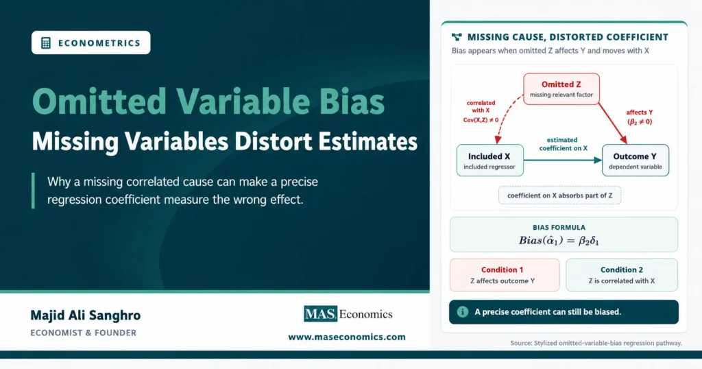
The bias pathway can be summarized as a simple causal structure. The omitted variable affects the outcome and is also correlated with the included regressor. The regression then assigns part of the omitted variable’s effect to the included variable.

The diagram shows why omitted variable bias is a pathway problem. The included variable \(X\) has an estimated path to the outcome \(Y\). The omitted variable \(Z\) also affects \(Y\), and it is correlated with \(X\). Leaving out \(Z\) makes the coefficient on \(X\) absorb part of the missing pathway.

Multiple regression reduces the risk

Multiple regression helps address omitted variable bias by adding relevant controls. If the omitted factor can be measured and included, the coefficient on \(X\) can be estimated while holding that factor constant.

The regression becomes:

Controlled regression

Now \(\beta_1\) measures the association between \(X\) and \(Y\) after controlling for \(Z\), conditional on the model being otherwise valid. This is one of the main reasons multiple regression is central in applied econometrics.

Controls should not be added mechanically. A control variable must be chosen because it belongs in the economic model. Adding bad controls can introduce new problems, especially if the control is itself caused by the variable of interest or lies on the causal pathway from \(X\) to \(Y\).

The purpose of controls is not to maximize the number of variables. It is to isolate the relationship of interest by accounting for relevant confounding factors.

Control variables need economic logic

Good control selection begins with the research question. A variable is a confounder when it affects the outcome and is related to the explanatory variable of interest. That is the variable type most relevant to omitted variable bias.

For example, in a regression of earnings on education, work experience may be a relevant control because experience affects earnings and may be related to education. Region may matter if labor markets differ geographically and education levels vary across regions. Family background may matter if it affects both educational attainment and wages.

But some variables should not be controlled for. If the goal is to estimate the total effect of education on earnings, controlling for occupation may remove part of the effect if education changes occupational choice. That would be overcontrol rather than correction.

Econometric judgment therefore requires a causal map. The model should identify which variables are confounders, which are outcomes of the treatment variable, and which are irrelevant background noise.

Direction depends on two signs

The sign of omitted variable bias depends on two relationships. The first is the relationship between the omitted variable and the outcome. The second is the relationship between the omitted variable and the included explanatory variable.

Table 1. Direction of omitted variable bias

Effect of omitted Z on Y	Correlation between Z and X	Bias in coefficient on X
Positive	Positive	Upward bias
Positive	Negative	Downward bias
Negative	Positive	Downward bias
Negative	Negative	Upward bias
Zero	Any correlation	No omitted-variable-bias channel
Central rule	Multiply the two signs	Bias direction follows \(\beta_2\delta_1\)
Source: MASEconomics editorial synthesis based on the standard omitted variable bias formula.

The table is useful because it prevents vague statements about bias. A missing variable does not always inflate a coefficient. It can also push the coefficient downward, and in some cases it may not bias the coefficient of interest at all.

Bias can hide or exaggerate effects

Omitted variable bias can make an effect look larger than it is. It can also make a real effect look smaller, zero, or even opposite in sign. The direction depends on the omitted factor and its relationship with the included variable.

Suppose a study estimates the effect of training on wages but omits motivation. If more motivated workers are more likely to attend training and motivation also raises wages, the training coefficient may be biased upward. The estimate may partly reflect motivation rather than training.

Now consider a pollution and house-price regression that omits distance to the city center. If polluted areas are closer to jobs and central locations raise house prices, the negative effect of pollution may be biased toward zero. The omitted location advantage masks part of the pollution discount.

These examples show why the sign of bias must be reasoned through case by case. The same econometric problem can exaggerate or conceal the relationship being studied.

Prediction and causality differ sharply

Omitted variable bias is most serious when the goal is causal interpretation. If the goal is prediction, leaving out a variable may still hurt accuracy, but the meaning of bias is different.

A forecasting model may perform well even if it does not include every causal variable, provided the included predictors contain enough information to predict the outcome. Prediction asks whether the model forecasts accurately. Causal inference asks whether the coefficient measures the effect of changing \(X\) while holding relevant confounders fixed.

For causal claims, omitted variable bias is dangerous because it changes the interpretation of the coefficient. The estimate no longer answers the intended causal question. It reflects both the included variable and the missing correlated determinant.

This is why applied econometric work often separates descriptive regression, predictive modeling, and causal estimation. The same regression table can serve different purposes only when its assumptions are clearly stated.

Fixed effects can remove some bias

Fixed effects can reduce omitted variable bias when the omitted factor is constant within an individual, firm, region, school, or country over time. By comparing changes within the same unit, fixed effects remove time-invariant unobserved differences.

For example, if unobserved ability is constant over time, an individual fixed-effect model can remove that fixed ability component. The coefficient is then identified from changes within the same person rather than differences across people.

But fixed effects do not solve every omitted variable problem. They do not remove omitted factors that change over time and are correlated with the variable of interest. They also do not fix measurement error, reverse causality, or omitted shocks that vary within the unit over time.

Fixed effects are therefore useful but conditional. They remove specific kinds of omitted variables, not all endogeneity.

Instrumental variables offer another route

When a relevant omitted variable cannot be measured, instrumental variables may help. An instrument is a variable that shifts the explanatory variable of interest but affects the outcome only through that explanatory variable, under the instrument’s assumptions.

The logic is to isolate variation in \(X\) that is not correlated with the omitted factor. If the instrument is valid and strong, the resulting estimate can avoid the omitted variable bias that affects ordinary least squares.

Instrumental variables are powerful but demanding. A weak instrument can produce unreliable estimates. An invalid instrument can create a different form of bias. The method depends on careful economic justification, not merely statistical convenience.

In practice, instrumental variables are used when ordinary controls are insufficient and a credible source of exogenous variation is available.

Experiments avoid the correlation problem

Randomized experiments are designed to avoid omitted variable bias by breaking the link between treatment assignment and omitted determinants of the outcome. If treatment is randomly assigned, observed and unobserved confounders should be balanced across treatment and control groups on average.

In that setting, the treatment variable is not systematically correlated with omitted factors. The estimated treatment effect is therefore not biased by the same omitted-variable pathway, assuming randomization is implemented correctly and attrition or noncompliance does not create new problems.

Natural experiments and quasi-experimental designs try to approximate this logic using policy changes, thresholds, lotteries, timing rules, or other institutional features. The goal is the same: find variation in \(X\) that is not driven by omitted determinants of \(Y\).

The deeper lesson is that omitted variable bias is about the source of variation. Reliable causal estimation requires variation in the explanatory variable that is not entangled with missing causes of the outcome.

Diagnostic tests cannot prove absence

There is no simple statistical test that proves omitted variable bias is absent. The omitted variable is missing by definition, so its full relationship with the included variable and the outcome cannot usually be tested directly.

Researchers often use indirect checks. They compare estimates across specifications, add plausible controls, test sensitivity to control groups, use fixed effects, or examine whether results change sharply when observed covariates are included.

These checks are useful, but they do not provide certainty. A coefficient that remains stable after adding controls is more reassuring than one that changes dramatically, but unobserved confounding may still remain.

The strongest defense is design-based. The study should explain why the remaining unobserved factors are unlikely to be correlated with the explanatory variable of interest, or it should use a research design that weakens that correlation.

Bad controls create new problems

Adding variables is not always an improvement. A bad control can distort the coefficient by blocking part of the causal effect or by opening a new source of bias.

One common mistake is controlling for a mediator. If education affects occupation and occupation affects earnings, then controlling for occupation removes part of the total effect of education. The coefficient on education then measures only a narrower direct effect, not the total effect.

Another mistake is controlling for a variable affected by both the treatment and unobserved determinants of the outcome. This can create collider bias. In that case, adding a control can make the regression worse, even though the model appears more complete.

The lesson is that controls need a causal reason. A longer regression is not automatically a better regression.

Standard errors cannot fix bias

Robust standard errors, clustered standard errors, and larger samples address inference problems, not omitted variable bias itself. They can make uncertainty estimates more appropriate, but they do not remove the correlation between the included regressor and the omitted factor.

This distinction matters in applied work. A coefficient can be statistically significant and biased. A regression can have robust standard errors and still suffer from omitted confounding. A large dataset can produce narrow confidence intervals around the wrong estimand.

The correction must target the source of bias. That may mean adding a relevant control, using fixed effects, changing the research design, applying instrumental variables, or narrowing the claim from causal to descriptive.

Standard errors answer a sampling question. Omitted variable bias is a specification and identification question.

Model transparency reduces confusion

A credible regression should state what coefficient is being interpreted and what assumptions are needed. If the coefficient is descriptive, the language should remain descriptive. If it is causal, the model must explain why omitted confounding is not driving the result.

One practical approach is to write the suspected true model before writing the estimated model. This makes omitted factors visible. It also helps identify which controls are essential, which are optional, and which may be bad controls.

Another approach is to report a sequence of specifications. A simple regression can show the raw association. Additional specifications can add controls, fixed effects, or alternative samples. If the coefficient changes substantially, that change itself is informative.

Transparency does not eliminate omitted variable bias, but it makes the risk easier to evaluate. It prevents a regression coefficient from being treated as causal without an argument.

Explains

Conclusion

Omitted variable bias occurs when a missing variable affects the dependent variable and is correlated with an included explanatory variable. The estimated coefficient then absorbs part of the missing variable’s effect, so it no longer cleanly measures the relationship of interest.

The bias formula \(\operatorname{Bias}(\hat{\alpha}_1)=\beta_2\delta_1\) shows why direction matters. A missing variable can push a coefficient upward or downward depending on its effect on the outcome and its relationship with the included regressor.

The solution is not mechanical variable collection. Reliable regression analysis requires economic reasoning, careful controls, credible research design, and honest interpretation of what the coefficient can support. Larger samples and robust standard errors improve precision and inference, but they do not repair a misspecified causal model.

Frequently Asked Questions

Did you find this article helpful? Share it with someone who loves economics. And remember, at MASEconomics, we make complex ideas simple.