Mastering Multiple Regression Models in Econometrics

Labor market data reveal that hourly wages depend on more than just years of education. Experience, geographic location, industry type, and union status also shape earnings. Multiple regression models isolate the effect of each explanatory variable while holding others constant. This technique transforms bivariate estimation into a multivariate framework, allowing economists to control for confounding factors and approximate causal effects more closely. Observational data lacks the randomized control of experimental settings, making multivariate controls the primary mechanism for isolating specific economic relationships. By introducing a matrix structure that partials out the influence of control variables, multiple regression reveals the direct relationship between a specific regressor and the outcome.

The Logic of Adding Control Variables

Bivariate estimation provides a useful starting point, but economic outcomes rarely stem from a single cause. When an unobserved variable correlates with both the dependent variable and the included regressor, the OLS estimator captures the combined effect, producing biased results. Multiple regression mitigates this problem by bringing those correlated factors directly into the equation.

Consider the relationship between education and wages. Innate ability correlates with both schooling and earnings. In a simple linear regression, the slope on education captures both the true return to schooling and the return to innate ability, overstating the effect. By adding a proxy for ability, such as a standardized test score, the multiple regression model isolates the pure effect of education. The resulting coefficient on education represents its effect holding test scores constant, providing a more accurate measure of the economic return to schooling.

The mathematical structure of omitted variable bias makes this clear. If the true population model includes two regressors, \( y = \beta_0 + \beta_1 x_1 + \beta_2 x_2 + v \), but the analyst estimates a short regression excluding \( x_2 \), the expected value of the estimated coefficient \( \tilde{\beta}_1 \) becomes:

The bias depends on two factors: the true effect of the omitted variable \( \beta_2 \), and the linear relationship between the included and omitted variables \( Cov(x_1, x_2) \). If ability positively affects wages and positively correlates with education, the bivariate estimate overstates the return to education. Multiple regression eliminates this specific bias by including \( x_2 \) in the estimation.

The conditional interpretation defines multiple regression. Each slope coefficient measures the expected change in the dependent variable associated with a one-unit increase in that specific independent variable, holding all other regressors fixed. This ceteris paribus condition is the defining feature of multiple regression, enabling analysts to disentangle overlapping relationships and estimate partial effects. The foundations of econometrics rely heavily on this conditional expectation framework to test economic theories against real data.

Matrix Algebra of the OLS Estimator

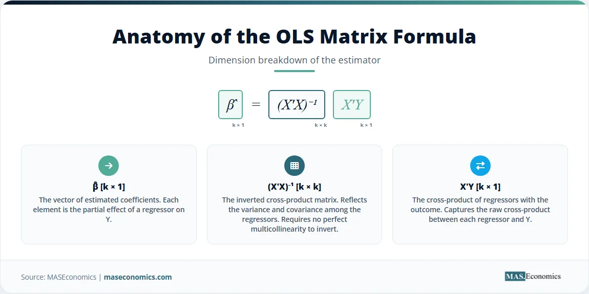
Multiple regression requires matrix algebra to handle several explanatory variables simultaneously. The population model expands to include \( k \) regressors and \( n \) observations. Let \( \mathbf{Y} \) denote the \( n \times 1 \) vector of dependent variable observations, \( \mathbf{X} \) the \( n \times k \) matrix of independent variables including a column of ones for the intercept, \( \mathbf{\beta} \) the \( k \times 1 \) vector of population coefficients, and \( \mathbf{\epsilon} \) the \( n \times 1 \) vector of error terms.

The OLS estimator \( \hat{\mathbf{\beta}} \) minimizes the sum of squared residuals. The residual vector \( \hat{\mathbf{u}} \) is the difference between the observed and predicted values.

The objective function in matrix form minimizes the quadratic form of the residuals.

Taking the derivative with respect to \( \hat{\mathbf{\beta}} \) and setting it equal to zero yields the first-order condition.

Expanding the terms and rearranging gives the normal equations in matrix form. Assuming \( \mathbf{X}’\mathbf{X} \) is invertible, meaning no perfect multicollinearity exists, solving for \( \hat{\mathbf{\beta}} \) produces the OLS estimator formula.

This formula generates the vector of estimated coefficients. The variance-covariance matrix of the estimator quantifies the uncertainty around these estimates. Under the assumption of homoscedasticity, the variance-covariance matrix depends on the error variance \( \sigma^2 \) and the matrix of regressors.

Since the true error variance is unknown, analysts estimate it using the variance of the residuals. The unbiased estimator of \( \sigma^2 \) divides the sum of squared residuals by the degrees of freedom, \( n – k \). Under the Gauss-Markov assumptions, the matrix OLS estimator is BLUE, providing the most efficient linear unbiased estimates of the population parameters. When heteroscedasticity is present, the standard formula for the variance becomes invalid, requiring robust covariance matrices to correct the inference.

The Frisch-Waugh-Lovell theorem provides the mathematical foundation for the holding constant interpretation. The theorem states that the sub-vector \( \hat{\mathbf{\beta}}_1 \) from the multiple regression of \( \mathbf{Y} \) on \( \mathbf{X}_1 \) and \( \mathbf{X}_2 \) is numerically identical to the coefficient obtained from a simple regression of \( \mathbf{Y} \) on the residuals of \( \mathbf{X}_1 \), where those residuals come from a regression of \( \mathbf{X}_1 \) on \( \mathbf{X}_2 \). Let \( \mathbf{M}_2 = \mathbf{I} – \mathbf{X}_2(\mathbf{X}_2’\mathbf{X}_2)^{-1}\mathbf{X}_2′ \) be the annihilator matrix for \( \mathbf{X}_2 \). The FWL estimator is:

This demonstrates that multiple regression mechanically purges the linear influence of the control variables from both the dependent variable and the regressor of interest before estimating the slope. The partial regression plot visualizes exactly this mathematical operation.

Goodness of fit in the multivariate framework extends the bivariate R-squared. The coefficient of determination measures the fraction of the sample variance in \( \mathbf{Y} \) explained by the regressors.

Because adding variables never increases the sum of squared residuals, \( R^2 \) mechanically rises with every added regressor, even irrelevant ones. Adjusted R-squared penalizes this inflation by accounting for the degrees of freedom.

This adjustment ensures that adding a variable only improves the metric if its explanatory power exceeds the penalty for losing a degree of freedom, providing a more reliable metric for comparing models with different numbers of regressors.

Interpreting OLS Results: Wages on Education

Returning to the wage example, expanding the model to include years of experience alongside education provides a clearer picture of labor market dynamics. The OLS estimation yields an intercept of 3.10, an education coefficient of 0.95, and an experience coefficient of 0.45. The estimated equation becomes:

In multiple regression, the intercept represents the expected value of the dependent variable when all regressors equal zero. An intercept of 3.10 implies a base wage of $3.10 per hour for an individual with zero education and zero experience. While this specific extrapolation rarely holds practical meaning, it anchors the regression plane in the data space. The education coefficient of 0.95 means that each additional year of schooling is associated with a $0.95 increase in hourly wages, holding experience constant. The experience coefficient of 0.45 means that each additional year of experience is linked to a $0.45 increase in hourly wages, holding education constant. Comparing this to the bivariate estimate, where the return to education was $1.20, the drop to $0.95 reflects the omitted variable bias in the simple regression, where education absorbed some of the positive effect of experience.

Table 1 reports the full output. Both regressors carry three significant stars, confirming their statistical importance. The R-squared increases from 0.340 in the bivariate model to 0.410 in the multiple regression, showing that adding experience explains additional variation in wages. The F-statistic of 68.10 tests the joint null hypothesis that all slope coefficients are equal to zero. Rejecting this hypothesis confirms that the model possesses significant explanatory power.

Table 1. OLS Estimation: Hourly Wages on Education and Experience

Variable	Coefficient	Std. Error	t-statistic	p-value
Intercept	3.10***	(0.90)	3.44	<0.001
Education (years)	0.95***	(0.15)	6.33	<0.001
Experience (years)	0.45***	(0.08)	5.62	<0.001
R-squared	0.410
Adj. R-squared	0.405
F-statistic	68.10 (p < 0.001)
Observations	198

Note: ^* p<0.10, ^** p<0.05, ^*** p<0.01. Standard errors in parentheses. Stylized canonical example.

The partial regression plot visualizes the independent effect of education. It displays the relationship between wage residuals and education residuals, both purged of the linear influence of experience. This plot represents the Frisch-Waugh-Lovell theorem visually. The upward slope confirms the positive partial effect of schooling, showing the holding constant mechanism. The slope of the line through these residualized points precisely matches the 0.95 coefficient on education in the full multiple regression.

Joint hypothesis testing extends inference beyond individual coefficients. An analyst might test whether the returns to education and experience are jointly equal to specific values predicted by economic theory. The F-test compares the sum of squared residuals from the restricted model to the unrestricted model. In the wage regression, the F-statistic overwhelmingly rejects the null that neither education nor experience affects wages, validating the multivariate framework.

Wage Gaps and GDP Growth in the Multivariate Lens

Multiple regression anchors empirical research across macroeconomics, finance, and program evaluation. The IMF World Economic Outlook relies on multivariate models to estimate the determinants of cross-country GDP growth. Analysts include investment rates, population growth, initial income levels, and institutional quality indices. The coefficient on investment isolates the effect of capital accumulation on growth, controlling for demographic and institutional differences. Without these controls, the investment coefficient would capture the fact that countries with strong institutions both invest more and grow faster, conflating the institutional effect with the capital effect.

Labor economists use multiple regression to measure the gender wage gap. A National Bureau of Economic Research study regresses log wages on a gender indicator, education, experience, occupation, and industry dummies. The coefficient on the female indicator measures the residual wage gap not explained by observable productivity characteristics. This approach reveals whether wage disparities stem from different career choices or from systemic pay discrimination. The World Bank gender data relies on similar models to track global progress on wage equality.

Central banks depend on multivariate models for monetary policy. The Federal Reserve estimates the natural rate of unemployment using models that include inflation, lagged unemployment, labor market tightness, and structural policy variables. The Bank for International Settlements uses multiple regression to model the drivers of sovereign bond yields, including debt-to-GDP ratios, global risk indices, liquidity measures, and credit ratings. When evaluating fiscal policy, researchers at the OECD Economics Department regress government spending multipliers on initial debt levels, trade openness, exchange rate regimes, and monetary policy stance. These multivariate frameworks control for confounding macroeconomic conditions, yielding more reliable policy conclusions than bivariate estimates.

Health economics also relies on multivariate controls. Researchers estimating the effect of health insurance on medical utilization must control for income, age, chronic conditions, and regional healthcare prices. Without these controls, the estimated effect of insurance captures the fact that healthier, wealthier individuals both purchase more insurance and utilize more preventive care. Multiple regression isolates the pure access effect of insurance coverage from these confounding variables. When observational data suffers from endogeneity, analysts turn to instrumental variables or causal inference methods to isolate the true effect.

Where the Multivariate Framework Fails

Adding more variables does not automatically improve a model. Including irrelevant regressors reduces the degrees of freedom and increases the variance of the remaining estimators, making the estimates less precise. Model selection criteria like AIC and BIC penalize excessive complexity, helping analysts balance goodness of fit with parsimony.

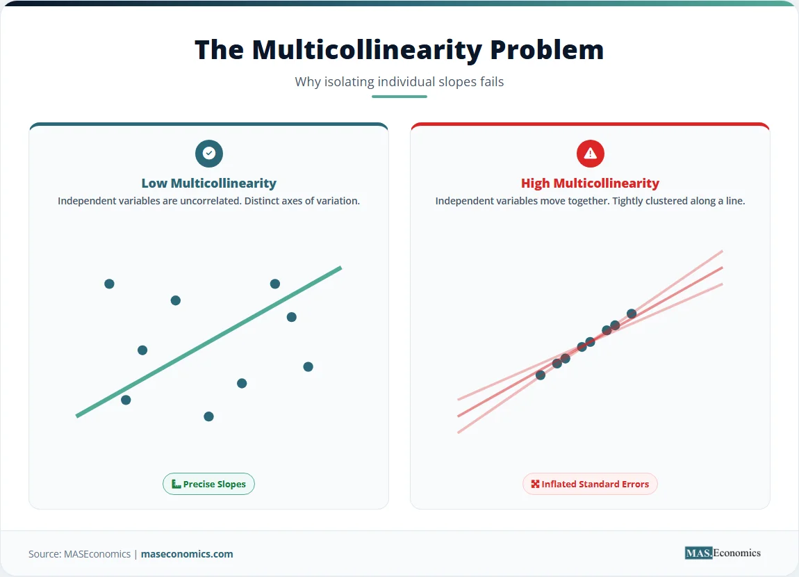
Multicollinearity occurs when two or more independent variables are highly correlated. This correlation inflates the standard errors, making it difficult to distinguish the individual effect of each regressor. In the wage example, if experience and age are both included, their high correlation makes their individual coefficients unstable. Detecting multicollinearity requires variance inflation factor diagnostics. The coefficients remain unbiased, but the wide confidence intervals render hypothesis testing unreliable. In extreme cases of perfect multicollinearity, the matrix \( \mathbf{X}’\mathbf{X} \) becomes singular, and the OLS estimator does not exist.

Functional form misspecification arises when the linear model misrepresents the true relationship. If the effect of experience on wages diminishes over time, including a linear term alone forces a constant slope, biasing the estimates. Adding polynomial terms or using logarithmic transformations can correct this issue. The Ramsey RESET test detects functional form problems by evaluating whether powers of the fitted values improve the model. The test regresses the dependent variable on the original regressors alongside the fitted values raised to increasing powers. If the coefficients on these powered terms are jointly significant, the model suffers from functional form misspecification, indicating that nonlinear combinations of the existing variables better explain the variation in the dependent variable.

Heteroscedasticity violates the constant variance assumption of the classical linear model. While the OLS coefficients remain unbiased, the standard errors become inconsistent, leading to invalid t-statistics and confidence intervals. Detecting heteroscedasticity involves the Breusch-Pagan test or White’s test. Correcting the inference requires heteroscedasticity-consistent standard errors, which adjust the variance-covariance matrix without changing the point estimates.

The OLS estimator also assumes strict exogeneity. If an unobserved variable correlates with a regressor but cannot be included, the estimates suffer from endogeneity. In such cases, the multivariate framework requires extensions like the generalized method of moments or natural experiments to recover consistent estimates.

MASEconomics Explains

Conclusion

Multiple regression models extend the bivariate framework by estimating the partial effect of several independent variables on a dependent variable. The matrix formulation of OLS provides a compact method for calculating coefficients, standard errors, test statistics, and confidence intervals. By holding other factors constant, multiple regression mitigates omitted variable bias and reveals direct relationships. The technique requires vigilance regarding multicollinearity, functional form misspecification, strict exogeneity, and the inclusion of bad controls. When these assumptions hold, the multivariate framework offers a powerful tool for policy evaluation and economic forecasting.

Thank you for reading! If you found this helpful, share it with friends and spread the knowledge. Happy learning with MASEconomics