Standard Errors Explained: Measuring Estimation Uncertainty

Every regression table has two columns that matter, and readers reliably fixate on the wrong one. The coefficient answers the question the study was run for: how big is the effect. The number beside it answers the question that decides whether the first answer is worth anything: how well do we actually know that. Standard errors measure the sampling uncertainty of an estimate, how much the coefficient would bounce around if the same study were rerun on fresh samples from the same world, and they are the raw material of every confidence statement, every significance star, and every honest sentence about what the data show. They are also where empirical work most often goes quietly wrong, because the default formula printed by every statistics package is built on assumptions that economic data routinely violate, and a wrong standard error corrupts every conclusion downstream while the coefficient sits there looking exactly the same.

The Spread of an Estimate, Not the Spread of the Data

The concept begins with an imagined experiment. Draw a sample, run the regression from our guide to simple linear regression, record the slope; now draw another sample from the same population and do it again, and again. The slopes differ from draw to draw, because each sample contains different noise, and the distribution of those slopes across hypothetical repetitions is the estimator’s sampling distribution. The standard error is that distribution’s standard deviation: the typical distance between one sample’s estimate and the truth. Every use made of it, the plus-or-minus-two rule for intervals, the coefficient-over-standard-error ratio behind test statistics in hypothesis testing, is a way of asking how far from the truth this one sample’s answer could plausibly sit.

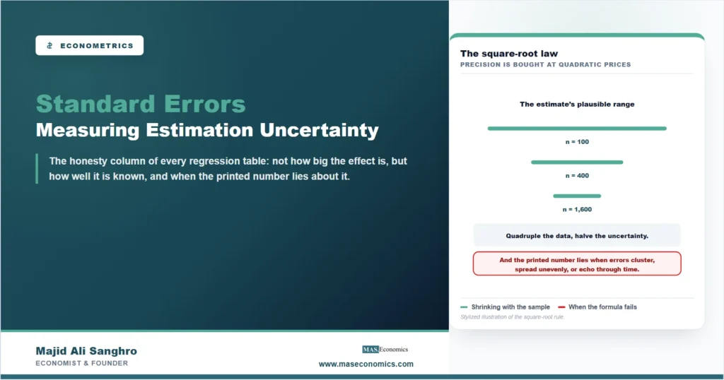
The classic confusion is with the standard deviation of the data, and the two answer different questions entirely. The standard deviation of wages describes how much wages vary across people, a fact about the world that no amount of sampling changes. The standard error of an estimated wage effect describes how precisely the study has pinned that effect down, and it shrinks as evidence accumulates, at the square-root rate: four times the observations buy half the standard error. That square-root arithmetic is worth internalizing, because it prices research designs, halving uncertainty costs quadruple data, and because it explains the modern landscape in one line: in the enormous samples now common, standard errors become tiny, everything becomes significant, and the interesting questions move from whether an effect exists to how large it is, exactly the shift the sample-size discussion in our p-values companion piece describes for testing.

When the Printed Number Lies

The default standard error is computed from a formula, and the formula embeds assumptions about the errors around the regression line: that they share one variance and do not lean on each other. Economic data violate both habitually, and each violation makes the printed number wrong in a known direction. When error variance grows with income, firm size, or scale, the condition treated in our article on heteroscedasticity, the default formula misprices the noise; the standard repair, heteroskedasticity-robust standard errors, recomputes the uncertainty without the equal-variance assumption and is now the reflexive default in applied microeconomics. When errors echo through time, this quarter’s shock persisting into the next, the default treats each observation as fresh information when it is partly a rerun, and the reported standard errors can be dramatically too small, the trap dissected in our guide to autocorrelation.

The modern extension of the same logic is clustering. In the grouped data of applied economics, workers within firms, students within schools, households within villages, observations inside a group share unmeasured influences, so a dataset of ten thousand students in fifty schools contains far fewer than ten thousand independent pieces of information about a school-level policy. Clustered standard errors compute uncertainty at the level where independence is credible, the fifty schools, and the correction routinely multiplies standard errors severalfold, which is why the choice of clustering level is among the most consequential lines in a modern empirical paper, especially in the panel data settings where the same units repeat over time. And when no formula can be trusted, because the estimator is exotic or the sample small, the uncertainty can be measured empirically by resampling the data itself, the approach explained in our article on bootstrap methods. The common thread is worth stating plainly: these corrections change no coefficient. They change how much the study claims to know, which is often the more consequential edit.

Reading the Second Column First

For a consumer of empirical work, three habits capture the practical value. First, read the standard error as a claim about evidence quality and check whether its construction matches the data’s structure: time series with default errors, grouped data clustered at a conveniently forgiving level, or a paper whose conclusions survive only under one choice of correction are all warnings written in the second column. Second, use the square-root rule to calibrate expectations: precision is bought with quadratic effort, so a small study claiming razor-sharp estimates deserves suspicion, and a large one waving significance around deserves the magnitude question instead. Third, remember what the number cannot do. A standard error measures sampling noise around whatever the regression is estimating; it is silent on whether the estimand means what the author claims, which is the identification territory of our article on instrumental variables. A biased estimate with a beautiful standard error is a precisely measured wrong answer, and no correction in this family fixes it.

MASEconomics Explains

Conclusion

Standard errors are the regression table’s honesty column: the estimated spread of the estimate itself across hypothetical repetitions, the input from which every interval and every star is manufactured, and the number that separates a measured claim from a guess wearing decimals. Their logic is sampling logic, their arithmetic obeys the square-root law that makes precision expensive, and their integrity depends entirely on whether the formula behind them matches the structure of the data, a match that heteroscedasticity, serial correlation, and clustering each break in well-mapped ways with well-mapped repairs.

The mature habit is to treat the second column as the first: before asking how big an effect is, ask how well it is known, whether the uncertainty was computed honestly for this kind of data, and whether the precision on offer is the kind sample size can buy or the kind only a sound design can. The corrections that occupy so much of applied econometrics never move a coefficient; they discipline what the coefficient is allowed to claim. That discipline is most of what separates empirical economics from arithmetic with opinions.

Frequently Asked Questions

Thanks for reading! The coefficient tells you the answer; the standard error tells you whether anyone should believe it. Happy learning with MASEconomics