Every time an econometrician fits a logit model, estimates a GARCH process, runs a Tobit regression, or trains a structural model of consumer choice, the same engine is doing the work in the background: maximum likelihood estimation. It is the workhorse method behind most non-OLS estimators in modern economics. The intuition is simple. Given a sample of data and an assumed probability model, choose the parameter values that make the observed data look as likely as possible. The mechanics, however, reward careful attention, because likelihood-based inference has its own assumptions, its own asymptotic theory, and its own pathologies when the model is wrong.
The Likelihood Principle
Start with a sample \( y_1, y_2, \ldots, y_n \) drawn independently from a distribution with density \( f(y; \theta) \), where \( \theta \) is the parameter vector to be estimated. The joint density of the sample, viewed as a function of \( \theta \) with the data held fixed, is called the likelihood function:
The likelihood is not a probability over \( \theta \). The data are fixed, observed quantities. The likelihood ranks how plausible different parameter values are at producing that fixed sample. Higher likelihood means the data are more consistent with that value of \( \theta \).
Because products of small numbers become numerically unstable, and because logarithms turn products into sums, almost all practical work uses the log-likelihood:
The maximum likelihood estimator, denoted \( \hat{\theta}_{MLE} \), is the value of \( \theta \) that maximises this function:
MLE of the Normal Mean and Variance
Suppose a sample of \( n \) observations is drawn from a normal distribution with unknown mean \( \mu \) and unknown variance \( \sigma^2 \). The density of each observation is:
Taking the log of the joint density across all \( n \) observations gives the log-likelihood:
To find the maximum, take partial derivatives with respect to \( \mu \) and \( \sigma^2 \) and set them to zero. The first-order condition for \( \mu \) gives:
The MLE of the mean is the sample average, which coincides with the OLS estimator and the method-of-moments estimator. The first-order condition for \( \sigma^2 \) gives:
Notice the denominator is \( n \), not \( n – 1 \). The MLE of the variance is biased in finite samples. It systematically underestimates the true variance because it divides by \( n \) instead of correcting for the degrees of freedom used in estimating the mean. The unbiased sample variance with \( n – 1 \) in the denominator is the method-of-moments correction, not the MLE. This is the first useful lesson: MLE is not guaranteed to be unbiased. Its appeal lies elsewhere, in its large-sample properties.
A Numerical Illustration
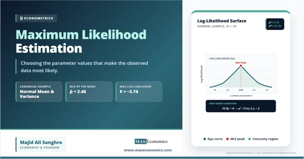
Consider a stylized sample of monthly inflation rates for a small open economy, with \( n = 10 \) observations: 2.1, 2.4, 1.9, 2.8, 3.1, 2.6, 2.2, 2.7, 2.5, 2.3. Apply the maximum likelihood formulas directly.
| Quantity | Formula | Value |
|---|---|---|
| Sample size | \( n \) | 10 |
| MLE of the mean | \( \hat{\mu} = \frac{1}{n}\sum y_i \) | 2.460 |
| Sum of squared deviations | \( \sum (y_i – \hat{\mu})^2 \) | 1.244 |
| MLE of the variance | \( \hat{\sigma}^2 = \frac{1}{n}\sum (y_i – \hat{\mu})^2 \) | 0.1244 |
| MLE of the standard deviation | \( \hat{\sigma} = \sqrt{\hat{\sigma}^2} \) | 0.353 |
| Unbiased variance (for comparison) | \( s^2 = \frac{1}{n-1}\sum (y_i – \hat{\mu})^2 \) | 0.1382 |
| Maximised log-likelihood | \( \ell(\hat{\mu}, \hat{\sigma}^2) \) | -3.74 |

The MLE variance of 0.1244 is noticeably smaller than the unbiased sample variance of 0.1382. The gap is the small-sample bias. For \( n = 10 \) the bias is roughly 10 percent. For \( n = 1000 \) it would be 0.1 percent. As the sample grows, the two estimators converge, and the bias becomes irrelevant.
Visualising the Log-Likelihood Surface
Holding the variance at its MLE value of 0.1244 and varying the mean \( \mu \), the log-likelihood traces a concave curve that peaks at the sample mean. The same logic applies to the variance dimension. The maximum is the highest point of a bowl-shaped surface in two-parameter space. The curvature of that surface at the peak carries information about precision: a steep curvature means small changes in \( \theta \) sharply reduce likelihood, which signals a precisely estimated parameter. A flat curvature signals weak identification.
This curvature is formalised by the Fisher information, defined as the negative expected second derivative of the log-likelihood:
The inverse of the Fisher information gives the asymptotic variance of the MLE. In practical work, the observed information, evaluated at \( \hat{\theta} \), is used.
Asymptotic Properties of the MLE
The reason maximum likelihood estimation became the default for non-linear models is not finite-sample performance. It is the package of asymptotic properties that hold under regularity conditions. As the sample size grows:
Consistency. The MLE converges in probability to the true parameter value. Formally, \( \hat{\theta}_{MLE} \xrightarrow{p} \theta_0 \). The estimator does not wander away from the truth as data accumulate.
Asymptotic normality. The distribution of the scaled estimator approaches a normal distribution centred at the true value:
This is what allows analysts to construct standard errors, confidence intervals, and Wald tests around MLE estimates.
Asymptotic efficiency. Among all consistent and asymptotically normal estimators, MLE achieves the smallest possible variance, the Cramér-Rao lower bound. No other estimator in this class can be more precise in large samples.
Invariance. If \( \hat{\theta} \) is the MLE of \( \theta \), then \( g(\hat{\theta}) \) is the MLE of \( g(\theta) \) for any well-defined function \( g \). Estimating \( \sigma^2 \) by MLE automatically gives the MLE of \( \sigma \) by taking the square root.
These properties depend on regularity conditions: the parameter space is open, the log-likelihood is differentiable, the true parameter lies in the interior, the model is correctly specified, and the Fisher information is finite and positive definite. When these fail, MLE can break in interesting ways.
Likelihood‑Based Hypothesis Tests
Maximum likelihood gives rise to a triad of asymptotically equivalent test statistics for testing \( H_0: \theta = \theta_0 \) against an alternative.
The likelihood ratio test compares the maximised log-likelihood under the null and the alternative:
where \( q \) is the number of restrictions. The Wald test uses the estimated parameter and its asymptotic variance:
The Lagrange multiplier test, also called the score test, uses the gradient of the log-likelihood evaluated at the restricted estimate:
where \( s(\theta) = \partial \ell / \partial \theta \) is the score. All three statistics share the same asymptotic chi-squared distribution and the same large-sample power. In finite samples, they often disagree, sometimes by enough to flip a conclusion.
Where MLE Lives Inside Modern Econometrics
The normal-mean example is pedagogical. The interesting applications appear once the model is non-linear in the parameters or the dependent variable is non-continuous. In a logit or probit model, the dependent variable is binary, and OLS is not appropriate. The log-likelihood for the logit becomes:
where \( \Lambda(\cdot) \) is the logistic CDF. There is no closed-form solution; the maximum is found numerically using Newton-Raphson or BHHH iterations. Tobit, Poisson, ordered probit, multinomial logit, duration models, and stochastic frontier models all rely on the same machinery. So do GARCH models of financial volatility and the Kalman filter step inside state-space models. Even ARMA estimation is most often done by exact or conditional maximum likelihood.
Compared with simple linear regression and multiple regression, where OLS provides a closed-form solution, MLE extends the toolkit to settings where linearity and continuity fail.
When the Likelihood Misleads
The asymptotic guarantees of MLE assume the model is correctly specified. Three failure modes recur in applied work.
Misspecification of the distribution is the most common. If a researcher assumes normality but the true errors are heavy-tailed or skewed, the MLE remains consistent for the parameter values that minimise the Kullback-Leibler divergence between the assumed and the true distribution, but it is no longer efficient, and its standard errors are biased. The remedy is the quasi-maximum-likelihood estimator with robust sandwich standard errors, or a different distributional assumption altogether.
Weak identification occurs when the log-likelihood is nearly flat in some direction. Parameters that are technically identified become statistically unidentifiable in finite samples. Standard errors balloon, and the asymptotic normality approximation fails. This is common in non-linear models with insufficient variation in regressors.
Boundary problems arise when the true parameter sits on the boundary of the parameter space. Variance components that should be non-negative, or autoregressive coefficients near unity, violate the regularity condition that the true parameter lies in the interior. The standard chi-squared distribution of the likelihood ratio test no longer applies, and inference requires non-standard distributions.
Finally, the choice of starting values matters in non-linear maximisation. A poorly chosen starting value can lead the optimiser to a local maximum rather than the global one. Practical work uses multiple starts and sensitivity checks.
Comparison with OLS, GMM, and Bayesian Methods
OLS is the maximum likelihood estimator for the linear regression model with normally distributed errors. In that special case, the two methods coincide. Once normality fails or the model becomes non-linear, the methods diverge.
Method of moments matches sample moments to population moments. It is often simpler and does not require a distributional assumption, but it is rarely efficient.
The generalised method of moments extends the method of moments by exploiting more moment conditions than parameters. It is the standard approach when distributional assumptions are unattractive, such as in much of instrumental variables estimation.
Bayesian estimation combines the likelihood with a prior distribution over parameters. With a flat prior, the Bayesian posterior mode equals the MLE. With informative priors, the two diverge in finite samples but typically converge as the sample grows.
Bootstrap methods are often used to construct standard errors and confidence intervals for MLE estimates in finite samples, especially when the asymptotic normal approximation is suspect.
MASEconomics Explains
Three ideas that frame maximum likelihood estimation
Explore more econometric methods and how they connect to applied economic research.
Explore the MASEconomics BlogPractical Estimation Guidelines
Three habits separate careful MLE work from automated runs. First, write down the log-likelihood explicitly before estimating, and check that the assumed distribution is plausible for the data. Second, report not only the point estimate but the maximised log-likelihood, the gradient at the optimum, and the eigenvalues of the Hessian, so that convergence and identification can be assessed. Third, accompany Wald standard errors with likelihood-ratio or bootstrap intervals when the sample is small or the surface is non-quadratic. Model selection across competing likelihood-based specifications uses information criteria such as AIC and BIC, both of which are penalised functions of the maximised log-likelihood.
Frequently Asked Questions
What is the difference between OLS and maximum likelihood estimation?
OLS minimises the sum of squared residuals; MLE maximises the likelihood of the observed data given a probability model. For a linear regression with normally distributed errors, the two methods give identical point estimates for the slope coefficients. They diverge when the model is non-linear, when the dependent variable is binary or count-valued, or when errors are non-normal.
Why is the MLE of the variance biased?
The MLE divides the sum of squared deviations by \( n \), not \( n – 1 \). Because the sample mean is itself estimated, one degree of freedom is used up, and dividing by \( n \) understates the true variance in finite samples. The bias vanishes as \( n \) grows. The unbiased sample variance corrects for this by dividing by \( n – 1 \).
When does maximum likelihood fail?
MLE fails when the model is severely misspecified, when parameters are weakly identified, when the true parameter sits on the boundary of the parameter space, or when the optimiser converges to a local rather than global maximum. In these cases the asymptotic normal approximation may be unreliable, and inference based on it can be misleading.
What is the Fisher information used for?
The Fisher information measures the curvature of the log-likelihood at its maximum. Its inverse gives the asymptotic variance of the MLE, which is used to construct standard errors and confidence intervals. High curvature means precise estimation; low curvature signals weak identification.
Are the likelihood ratio, Wald, and Lagrange multiplier tests interchangeable?
They are asymptotically equivalent and share the same chi-squared distribution under the null. In finite samples they can differ noticeably. The likelihood ratio test requires estimating the model under both null and alternative; the Wald test only requires the unrestricted estimate; the Lagrange multiplier test only requires the restricted estimate. The choice depends on which is easier to compute.
Thanks for reading! If you found this helpful, share it with friends and spread the knowledge. Happy learning with MASEconomics