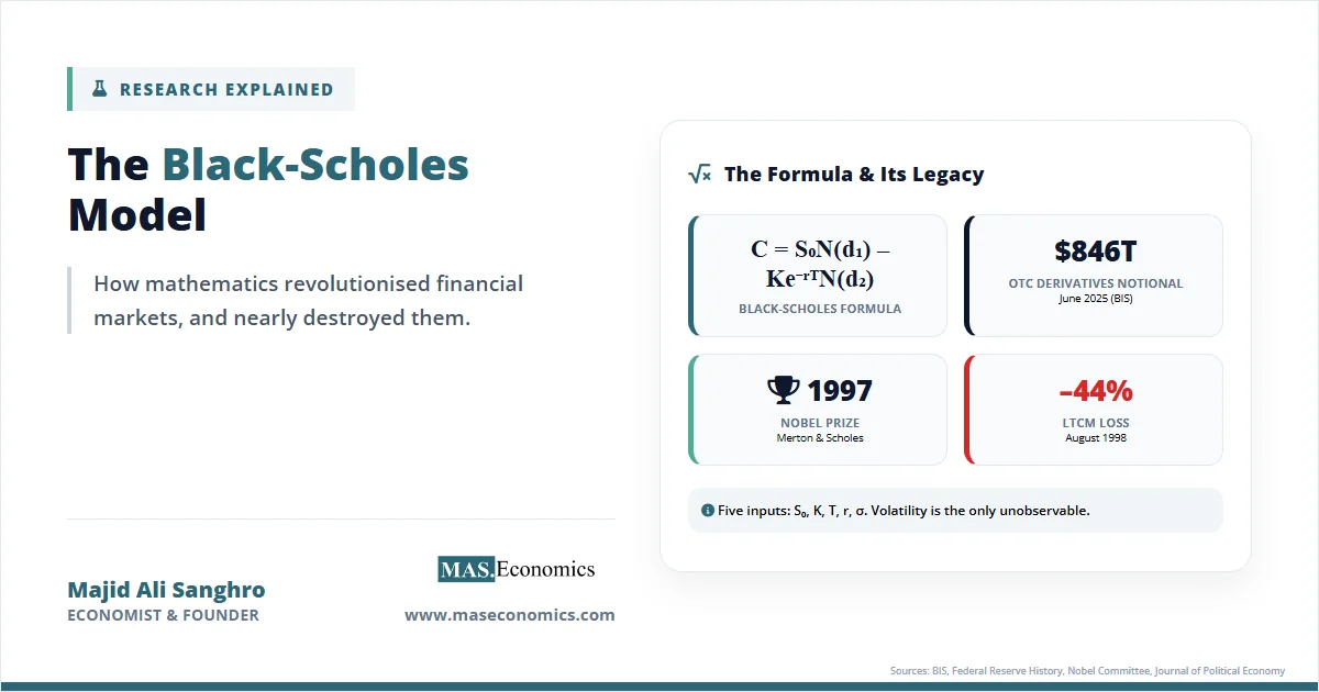
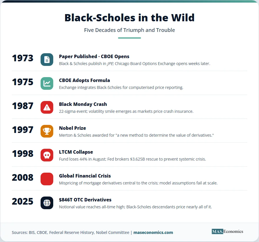
In the summer of 1973, two pages of equations in the Journal of Political Economy changed how the world values risk. The paper was titled “The Pricing of Options and Corporate Liabilities” by Fischer Black and Myron Scholes, and its argument was startling: the fair price of a stock option could be calculated from five observable inputs, with no guesswork about investor appetite for risk. The Black-Scholes model explained, at last, what generations of traders had tried to intuit on the floor. Within two years, the Chicago Board Options Exchange had adopted the formula for computerised price reporting, and the modern derivatives industry was born.
The puzzle Black and Scholes solved was old. An option is a contract giving the buyer the right, but not the obligation, to buy or sell an asset at a fixed price on a fixed date. Louis Bachelier had attempted a mathematical theory of options in his 1900 Paris dissertation. Paul Samuelson and Case Sprenkle refined the problem in the 1960s. All of them ran into the same wall: any valuation seemed to require knowing the expected return on the underlying stock, and expected returns depend on how much compensation investors demand for bearing risk, which nobody could measure cleanly.
Black and Scholes, working closely with Robert Merton, found a way around the wall. Their insight was that a trader holding an option could continuously adjust a position in the underlying stock so that the combined portfolio carried no risk at all. If the hedged portfolio is truly risk-free, it must earn the risk-free interest rate. Otherwise, arbitrage would be possible. That single no-arbitrage condition collapses the problem. The expected return on the stock drops out of the equation entirely, and the option price becomes a function of variables that can actually be observed or estimated. The Nobel Committee in 1997 cited this discovery as the breakthrough that separated the option from the risk of the underlying security, and awarded the prize to Merton and Scholes (Black had died in 1995 and the Nobel is not given posthumously).
The timing was almost theatrical. The Chicago Board Options Exchange opened on 26 April 1973, just weeks before the paper appeared. A market that began with 911 contracts on its first day now trades millions every session, and the intellectual architecture sitting behind it is the formula this article unpacks.
Black-Scholes Formula and Equations
The Black-Scholes derivation begins with an assumption about how stock prices move. The model treats the share price \( S_t \) as following geometric Brownian motion:
Here \( \mu \) is the drift (the expected rate of return), \( \sigma \) is the volatility (the standard deviation of returns), and \( dW_t \) is the increment of a standard Wiener process. Returns are normally distributed, prices are lognormal, and movements over non-overlapping intervals are independent.
The central trick is the construction of a riskless hedge. Consider a portfolio that is long one call option worth \( C \) and short \( \Delta \) shares of the underlying stock. Applying Itô’s lemma to \( C(S, t) \) and choosing \( \Delta = \partial C / \partial S \) eliminates the stochastic term. The portfolio is now locally riskless, so it must earn \( r \), the risk-free rate. Setting up that equality and rearranging yields the Black-Scholes partial differential equation:
With the boundary condition that at expiry the call is worth \( \max(S_T – K, 0) \), the PDE has a closed form solution. For a European call on a non-dividend-paying stock:
where
and \( N(\cdot) \) is the cumulative distribution function of the standard normal. The put price follows from put call parity: \( P = K e^{-rT} N(-d_2) – S_0 N(-d_1) \).
The formula is economic in its use of inputs. Five variables enter, four of them directly observable. The deep insight, discussed in the San Francisco Federal Reserve’s review of the 1997 Nobel, is that \( \mu \) never appears. Investor appetite for risk is already impounded in the current share price \( S_0 \). Once that price is observed, the option can be valued as if every investor were risk neutral, discounting at \( r \) rather than at a risk-adjusted rate. This is the risk-neutral pricing principle that now underlies nearly all of derivatives mathematics.
Table 1. The Five Inputs: What the Black-Scholes formula needs
| Symbol | Variable | Economic meaning | Observable? |
|---|---|---|---|
| \( S_0 \) | Spot price | Current market price of the underlying share | Yes, directly |
| \( K \) | Strike price | Price at which the option can be exercised | Yes, contractual |
| \( T \) | Time to expiry | Years until the option matures | Yes, contractual |
| \( r \) | Risk free rate | Continuously compounded return on a safe asset | Yes, from Treasury yields |
| \( \sigma \) | Volatility | Annualised standard deviation of log returns | No, must be estimated |

|
|||
Volatility is the single unobservable input, and that fact does most of the work in explaining both the model’s triumphs and its failures. Estimate \( \sigma \) well, and the formula produces a price within pennies of what the market quotes. Estimate it poorly, and losses accumulate quickly, because options are leveraged instruments whose value changes non linearly with the underlying.
Assumptions and Limitations of Black-Scholes
Every elegant model rests on assumptions, and Black-Scholes rests on several that are known to be false. Acknowledging this honestly is the starting point for any serious use of the formula.
The model assumes that stock returns are normally distributed and that volatility is constant through time. Actual return distributions have fatter tails. Extreme moves happen more often than a normal distribution predicts, as Benoit Mandelbrot argued decades before the 1987 crash produced a twenty-two standard deviation event that a normal model said should occur once in roughly the age of the universe. The model assumes continuous trading with no transaction costs, no taxes, no bid-ask spreads, and the ability to short the stock freely. It assumes the risk-free rate is known and constant, that the stock pays no dividends during the life of the option, and that the option is European, meaning it can be exercised only at expiry.
Each of these assumptions has been relaxed in subsequent research. Merton extended the formula to continuous dividend yields in 1973. Cox, Ross, and Rubinstein developed binomial trees in 1979 to price American-style options. Heston introduced stochastic volatility in 1993. Jump diffusion models add discrete shocks. What is remarkable is how resilient the original remains: traders still quote prices by inverting the Black-Scholes formula to back out an implied volatility, then adjust that number for known shortcomings. The formula has become a common language rather than a literal description of markets. A deeper treatment of the boundaries between theoretical elegance and empirical reality can be found in the MASEconomics article on risk, uncertainty, and insurance, which distinguishes the measurable risks the model captures from the Knightian uncertainty it silently ignores.
Empirical Evidence and Volatility Smile
Empirical tests of Black-Scholes have produced a consistent pattern: the formula works well near the money and for short-dated options, and less well for deep out of the money contracts and for long horizons. The most famous anomaly is the volatility smile. If the model were literally correct, options on the same stock with the same expiry but different strikes would all imply the same volatility. They do not. Following the October 1987 crash, implied volatility for low strike S&P 500 puts began trading at a persistent premium to at-the-money contracts, and the smile (or, more commonly for equity indices, a leftward skew) has never gone away.
What the smile reveals is that the market prices protection against crashes more expensively than a lognormal world would justify. Investors pay up for insurance against left-tail events because they know returns are not normal. Far from invalidating the model, this pattern is itself measured using Black-Scholes: the whole language of volatility surfaces exists only because practitioners agree on the formula as a common yardstick.
The chart below illustrates the core comparative statics of the model: how a European call price on an at-the-money stock evolves as expiry approaches, under three volatility regimes.
Source: MASEconomics calculation using the Black-Scholes formula. Spot price \( S_0 = 100 \), strike \( K = 100 \), risk free rate \( r = 5\% \). Prices shown for volatilities \( \sigma = 15\%, 25\%, 40\% \) across declining time to expiry.
Two patterns stand out. First, the call option value rises monotonically with volatility at every horizon. The \( \sigma = 40\% \) curve sits roughly double the \( \sigma = 15\% \) curve, even though both options have identical strikes, spots, and rates. Higher volatility means fatter tails, which raises the expected payoff of a capped loss instrument. Second, time decay is convex. An at-the-money call loses value slowly when expiry is distant and much faster in its final weeks. This is the famous \( \theta \) of options trading, and it is why sellers of short-dated options earn a steady premium in quiet markets and why buyers of long-dated options often find their bet working against them before the underlying ever moves.
Tests of the model against large panels of listed options have generally confirmed that Black-Scholes captures most of the cross-sectional variation in prices once implied volatility is allowed to differ across strikes and maturities. The closer the real world resembles the model’s assumptions (liquid markets, continuously tradable underlying, short horizons, near the money strikes), the tighter the fit.
Why Black-Scholes Matters
The practical reach of the Black-Scholes framework is difficult to overstate. The Bank for International Settlements reports that the notional value of outstanding over-the-counter derivatives reached $846 trillion at June 2025, up 16% year on year, the largest annual increase since before the 2008 crisis. The vast majority of this market exists because the Black-Scholes revolution made it possible to price, hedge, and therefore intermediate risks that previously had no measurable value. Corporate treasurers hedging foreign exchange exposure, airlines locking in fuel costs, lenders protecting against default, pension funds buying equity put options, all of them are operating in an intellectual universe created in 1973.
The model also reshaped corporate finance. The original paper was not called “The Pricing of Options” alone. It was called “The Pricing of Options and Corporate Liabilities,” because Black and Scholes recognised that equity in a levered firm is itself a call option on the firm’s assets struck at the face value of debt. That insight launched a generation of structural credit models and continues to underpin how banks assess corporate default risk. Every reader interested in how this connects to broader asset pricing should consult the companion piece on the Capital Asset Pricing Model, which is the other half of the intellectual foundation on which modern finance rests.
Regulation adopted the model as well. The Basel Committee’s capital rules, the accounting standards under IFRS 13 and ASC 820 that govern fair value measurement, and the disclosure frameworks for executive stock compensation all rely on Black-Scholes or direct descendants of it. When a United States public company reports the grant date fair value of employee stock options in its 10 K, that number is almost always produced by a Black-Scholes variant. When a United Kingdom pension scheme marks to market its interest rate swaps, the discount curves and volatility surfaces sit on top of the same framework. Canada’s OSFI and the Australian Prudential Regulation Authority use derivative valuations anchored to the same mathematics when setting bank capital requirements.
The model’s dark side is equally well documented. Long Term Capital Management, the hedge fund co-founded by Scholes and Merton, lost 44 per cent of its value in August 1998 alone after Russia devalued the rouble and defaulted on domestic debt. Spreads that the fund’s models said should converge instead diverged. On 23 September 1998, the Federal Reserve Bank of New York organised a $3.625 billion recapitalisation by fourteen major creditors to prevent a disorderly liquidation. The fund had been leveraged at roughly twenty-five to one. The statistical models assumed that correlations across positions were stable; the crisis revealed they were not. Liquidity itself vanished as a pricing input during the flight to quality.
Almost exactly a decade later, the pattern repeated at a civilisational scale. The 2008 financial crisis saw the mispricing of mortgage-linked derivatives on a trillion-dollar scale. Mathematician Ian Stewart wrote that the Black-Scholes equation “underpinned massive economic growth” but was also “one ingredient in a rich stew of financial irresponsibility, political ineptitude, perverse incentives and lax regulation” that contributed to the crisis. The equation itself was not the problem. The problem was pretending that the assumptions held in conditions where they manifestly did not. Gaussian copulas used to price collateralised debt obligations assumed correlations drawn from placid periods; when housing prices fell nationally for the first time since the Depression, the models produced catastrophic underestimates of tail risk.
These failures have not retired Black-Scholes. They have changed how it is used. Modern desks layer volatility surfaces, jump components, and stochastic rates on top of the base framework. Regulators require stress testing against scenarios that violate the model’s assumptions. The link between rigorous pricing and rigorous risk management has become the core discipline of the industry, rather than a footnote. Readers interested in how this pricing machinery coexists with the broader question of whether markets aggregate information correctly should consult the MASEconomics article on the Efficient Market Hypothesis, which examines the assumption of no arbitrage from a different angle, and the deeper mathematical tools described in dynamic programming in economics.
The model also transformed academic finance itself. Before 1973, financial economics was largely verbal and descriptive. After 1973, it became a quantitative discipline in which rigorous arbitrage arguments carried real weight. Techniques developed for option pricing now appear in the valuation of real options on corporate investment projects, in the pricing of executive compensation, in the analysis of insurance products with embedded guarantees, in mortgage prepayment modelling, and in the pricing of catastrophe bonds. The connection between stochastic processes and economic decision making, once exotic, is now the lingua franca of top graduate programmes. Those new to these tools will find useful context in the MASEconomics introductions to game theory and strategic behaviour, and to information economics, both of which share the same no-arbitrage intellectual heritage.
Perhaps most importantly, Black-Scholes changed the meaning of risk in the economy. Before the model, risk was a qualitative attribute of an investment, discussed in the language of prudence and judgment. After the model, risk became a quantity: specifically, the volatility parameter \( \sigma \), with a visible market price attached. Treasurers could hedge it, pension funds could lay it off, and regulators could measure it. This quantification is the deep reason the derivatives market grew from a niche business into a structure larger than the real economy it was built to serve. Whether that transformation has been net beneficial remains one of the open questions of modern finance.
MASEconomics Explains
4 economic concepts behind the Black-Scholes model
Conclusion
The Black-Scholes model explained how to assign a consistent price to risk, and in doing so, it built the scaffolding of modern finance. Its assumptions are routinely violated, its predictions miss in the tails, and its misuse has contributed to some of the most expensive failures in financial history. Yet it remains the reference point from which every serious pricing discussion still begins. A formula that produces a number from five inputs, one of them not directly observable, should never have survived half a century of market stress. That it has done so is a testament both to the power of no arbitrage reasoning and to the humility with which the model must be applied. Mathematics revolutionised financial markets, but the revolution was never a guarantee against loss.
Did you find this article helpful? Share it with someone who loves economics. And remember, at MASEconomics, we make complex ideas simple.