Bordered Hessian: Second-Order Conditions

A firm choosing inputs under a cost constraint, a consumer maximizing utility under a budget constraint, or a planner optimizing welfare subject to a resource constraint all face the same mathematical issue: a first-order condition can identify a candidate point, but it does not prove that the point is a maximum or a minimum. The bordered Hessian is the matrix test used to check second-order conditions in constrained optimization.

The method matters because economic models often optimize with constraints. A household cannot spend beyond income. A firm cannot use more inputs than its technology and budget allow. A government cannot satisfy every policy target with limited resources. The bordered Hessian helps determine whether a candidate solution is locally consistent with the economic objective.

In mathematical economics, the bordered Hessian sits between differentiation, matrix algebra, and constrained optimization. It extends the ordinary Hessian test by adding the constraint’s derivatives to the curvature matrix.

First-order conditions find candidates

Constrained optimization begins with an objective function and a constraint. In a standard two-variable case, the problem can be written as:

Constrained optimization problem

The objective \(f(x,y)\) is optimized only over points that satisfy the constraint.

The usual method is to form a Lagrangian:

Lagrangian function

The first-order conditions set the partial derivatives of the Lagrangian equal to zero:

First-order conditions

These conditions identify a candidate optimum. They say that, at the chosen point, the objective’s marginal trade-off is aligned with the constraint’s marginal trade-off. In a consumer problem, the marginal rate of substitution equals the price ratio. In a producer problem, the marginal product trade-off matches the input-price ratio.

But the first-order conditions do not say whether the candidate is a constrained maximum, a constrained minimum, or a saddle point. That classification requires curvature. The bordered Hessian is the standard matrix device for checking that curvature when a constraint is present.

Curvature decides the local result

In unconstrained optimization, second-order conditions depend on the Hessian matrix of second derivatives. For a function \(f(x,y)\), the ordinary Hessian is:

Ordinary Hessian

The signs of the Hessian’s principal minors help classify curvature. A negative definite Hessian indicates local concavity and supports a maximum. A positive definite Hessian indicates local convexity and supports a minimum.

Constraints change the test because the optimizer is not free to move in every direction. Only movements along the constraint surface are feasible. The relevant curvature is therefore not the curvature of the objective over the entire plane. It is the curvature of the Lagrangian along feasible directions.

This is why the bordered Hessian adds a “border” around the second-derivative matrix. The border contains first derivatives of the constraint. These derivatives identify the feasible surface and make the matrix test account for the fact that only constraint-preserving changes are allowed.

The border comes from constraints

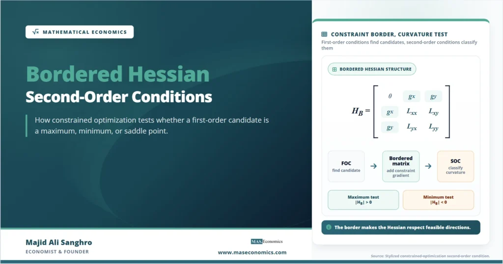
For one equality constraint with two choice variables, the bordered Hessian is:

Bordered Hessian matrix

The first row and column contain the constraint gradient. The lower-right block contains second derivatives of the Lagrangian with respect to the choice variables.

The zero in the top-left corner appears because the equality constraint itself has no second derivative with respect to the Lagrange multiplier in the relevant block. The entries \(g_x\) and \(g_y\) describe how the constraint changes when \(x\) or \(y\) changes. The entries \(\mathcal{L}_{xx}\), \(\mathcal{L}_{xy}\), \(\mathcal{L}_{yx}\), and \(\mathcal{L}_{yy}\) describe curvature of the Lagrangian.

The structure is easier to understand through the geometry. The constraint gradient points perpendicular to the feasible curve. The second-derivative block describes how the objective bends. The bordered Hessian combines both pieces so the second-order test is applied to feasible movements, not arbitrary movements.

The matrix form also shows why vectors and matrices are not decorative tools in economics. They compress a system of marginal and curvature conditions into a form that can be tested consistently.

The determinant carries the test

In the common two-variable, one-constraint case, the determinant of the bordered Hessian provides the key second-order test. The sign convention depends on how the Lagrangian is written, but with the structure above, a local constrained maximum typically requires:

Two-variable maximum test

A local constrained minimum typically requires:

Two-variable minimum test

The signs appear counterintuitive because the bordered Hessian is not the ordinary Hessian. The border changes the determinant’s sign pattern. The test is not asking whether the objective is concave or convex in all directions. It is asking whether curvature along the feasible set supports a maximum or minimum.

For more variables and constraints, the decision rule uses a sequence of bordered principal minors. The sign pattern depends on the number of choice variables, the number of constraints, and the convention used to define the Lagrangian. The essential idea remains the same: curvature must be checked only in directions that satisfy the constraint.

A utility example fixes intuition

Consider a consumer maximizing Cobb-Douglas utility subject to a budget constraint:

Consumer problem

The Lagrangian is:

The first-order conditions give the familiar tangency condition:

This condition says that the consumer’s marginal willingness to trade \(x\) for \(y\) equals the market’s price ratio. It identifies a candidate bundle on the budget line. The bordered Hessian then checks whether utility bends the right way along that budget line.

For Cobb-Douglas utility with positive \(x\) and \(y\), the indifference curves are convex to the origin and the utility function is concave over the relevant domain. The bordered Hessian test confirms that the tangency is a constrained maximum, not a minimum. Economically, the consumer chooses the highest reachable indifference curve, not merely any point where a slope condition holds.

The firm problem works similarly

The same structure appears in producer theory. A firm may minimize cost subject to producing a target output level:

Cost-minimization problem

The first-order conditions imply a tangency between the isoquant and the isocost line:

This is the same economic logic developed in optimization techniques. The first-order condition says that the technical trade-off between labor and capital equals the input-price trade-off. The firm has no local incentive to substitute one input for the other along the isoquant.

But the tangency alone does not prove cost minimization. The isoquant must have the correct curvature relative to the isocost line. The bordered Hessian verifies the second-order condition for a constrained minimum. In normal convex producer theory, it confirms that the chosen input mix is locally cost-minimizing.

The matrix generalizes cleanly

For \(n\) choice variables and one equality constraint, the bordered Hessian expands naturally. Let \(x=(x_1,\ldots,x_n)\), and let the constraint be \(g(x)=c\). The bordered Hessian has the form:

General one-constraint form

\(\nabla g(x)\) is the constraint gradient, and \(\nabla^2_{xx}\mathcal{L}\) is the Hessian of the Lagrangian with respect to the choice variables.

With several constraints, the top-left zero becomes a block of zeros, and the border contains the Jacobian matrix of all constraints. If there are \(m\) equality constraints and \(n\) choice variables, the structure is:

Multiple-constraint form

\(G_x\) collects the first derivatives of the constraints with respect to the choice variables.

This general form is why the bordered Hessian belongs in the mathematical economics toolkit. It combines the gradient logic of constraints with the curvature logic of second derivatives. The calculation becomes more complex as dimensions rise, but the economic interpretation remains tied to feasible curvature.

Decision rules depend on signs

The following table summarizes the intuition behind the common one-constraint test. It is deliberately presented as a guide to interpretation, not as a substitute for checking the sign convention used in a particular textbook.

Table 1. Bordered Hessian decision rules

Optimization case	Curvature requirement	Economic interpretation
Constrained maximum	Objective bends downward along feasible directions	The candidate sits on the highest nearby feasible objective value
Constrained minimum	Objective bends upward along feasible directions	The candidate sits on the lowest nearby feasible objective value
Saddle point	Curvature changes sign across feasible directions	The first-order condition holds, but the point is not a local optimum
Inconclusive test	Relevant determinant or minor equals zero	Higher-order or global analysis may be needed
Central rule	Check curvature on the constraint	The border makes the Hessian respect feasibility
Source: MASEconomics editorial synthesis based on standard constrained-optimization conditions.

The key message is not memorization of one isolated determinant sign. The key message is that first-order conditions locate candidates, while second-order conditions classify them. The bordered Hessian is the classification tool when equality constraints are present.

Equality constraints differ from inequalities

The bordered Hessian is mainly a tool for equality-constrained optimization. It fits problems where the constraint must hold exactly, such as a budget being fully spent or a required output level being produced.

Inequality constraints add another layer. A constraint such as \(x\geq 0\), \(g(x)\leq c\), or \(q\geq \bar{q}\) may bind or may not bind. If it binds, it behaves like an equality at the optimum. If it does not bind, it does not enter the local condition in the same way.

This is where Kuhn-Tucker conditions extend the logic. They combine first-order conditions, feasibility, complementary slackness, and sign restrictions on multipliers. For inequality-constrained problems, the bordered Hessian may still help after the active constraints have been identified, but it is not the whole test.

The distinction matters in economics. Many real problems involve corners. A consumer may buy none of one good. A firm may shut down a technology. A planner may hit a policy floor or ceiling. Equality-constrained curvature tests are useful, but they do not replace inequality analysis.

Local tests need global support

The bordered Hessian is a local test. It examines curvature near the candidate point. A local maximum is better than nearby feasible points, but it may not be the best feasible point over the entire domain.

Global conclusions need stronger structure. If the objective is concave and the constraint set is convex in a maximization problem, then a local maximum can also be global. If the objective is convex and the feasible set is convex in a minimization problem, then a local minimum can be global.

Without such structure, multiple local optima can exist. A bordered Hessian may classify one candidate correctly while another distant feasible point delivers a higher or lower objective value.

This is why second-order conditions should be read alongside the economic model. The shape of preferences, production sets, costs, and constraints determines whether a local result is enough.

Common errors distort conclusions

Several mistakes frequently lead to wrong bordered Hessian conclusions. The first is using the ordinary Hessian of the objective when the problem is constrained. That ignores feasible directions and can misclassify the candidate.

The second is using second derivatives of the objective \(f\) instead of second derivatives of the Lagrangian \(\mathcal{L}\). If the constraint is nonlinear, the second derivatives of the constraint affect the curvature of the Lagrangian and must be included.

The third is applying a sign rule without matching the Lagrangian convention. Changing from \(f+\lambda(c-g)\) to \(f-\lambda(g-c)\) can change signs in the matrix. The economic answer should be consistent, but the mechanical determinant rule must match the chosen form.

The fourth is treating a zero determinant as proof of failure. A zero determinant means the standard second-order test is inconclusive. Higher-order derivatives, global arguments, or a direct comparison of feasible objective values may be needed.

Economic applications are widespread

The bordered Hessian appears wherever economics uses constrained choice. Consumer theory uses it to verify utility maximization subject to a budget. Producer theory uses it to verify cost minimization or profit maximization with technological constraints. Welfare economics uses it in planner problems with resource constraints.

Macroeconomic models also use the same logic. A representative household may maximize lifetime utility subject to an intertemporal budget constraint. A firm may choose capital and labor subject to a production technology. A government may minimize a loss function subject to policy and feasibility constraints.

The common thread is not the specific field. The common thread is constrained curvature. When an economic agent chooses under a binding condition, first-order conditions give a candidate and the bordered Hessian helps verify the local nature of that candidate.

This makes the bordered Hessian a bridge between economic intuition and formal proof. It translates familiar ideas such as tangency, diminishing marginal utility, convex isoquants, and cost minimization into a matrix condition that can be applied across models.

Conclusion

Bordered Hessian analysis checks the second-order conditions for constrained optimization problems. It extends the ordinary Hessian by adding the derivatives of the constraint, so curvature is evaluated along feasible directions rather than over all possible movements.

The method clarifies a central distinction in economic modeling. First-order conditions identify candidate choices, but they do not classify them. The bordered Hessian helps determine whether the candidate is a local maximum, a local minimum, a saddle point, or an inconclusive case.

The test is powerful but conditional. Its sign rules depend on notation, the number of variables, the number of constraints, and the Lagrangian convention. Its result is local unless the economic model supplies global concavity, convexity, or other structure. Used carefully, it is one of the main tools connecting constrained choice to rigorous economic optimization.

Frequently Asked Questions

Thanks for reading! If you found this helpful, share it with friends and spread the knowledge. Happy learning with MASEconomics