Dummy Variables Regression: Categorical Effects Explained

A great deal of what economists want to explain is not a number. Whether a worker is unionized, which of four regions a firm operates in, whether a household owns its home, the industry a person works in, the season a sale occurs in: none of these is a quantity that can be plugged directly into a regression. Yet they often carry the most interesting variation in the data. The standard way to bring such categorical information into a regression is the dummy variable, a variable that takes the value one when a condition holds and zero when it does not. Dummy variables regression is the framework that lets qualitative, group-based information enter a model built for numbers, and it is one of the most widely used techniques in applied economics precisely because so much real-world variation is categorical.

The mechanics are simple to state and easy to get wrong. A dummy variable is just a column of zeros and ones, but the way those columns are constructed, how many to include, which category to leave out, and how to read the coefficients that result, trips up more empirical work than almost any other basic regression task. The recurring source of confusion is that a dummy coefficient is never a wage or a price on its own. It is always a comparison, measured against a category the model deliberately sets aside.

From a Category to a Column of Zeros and Ones

Consider the simplest case, a single two-way category such as union membership. Define a dummy variable equal to one for union members and zero for everyone else, and add it to a wage regression alongside education.

Single Dummy Variable

\(\text{union}_i = 1\) for union members, \(0\) otherwise. \(\beta_2\) is the wage difference between union and non-union workers at the same level of education.

The coefficient \(\beta_2\) does not describe union members in isolation. It describes the gap between union members and the group coded zero, holding education fixed. Writing the model out for each group makes this concrete. For non-union workers the dummy is zero, so the predicted wage is \(\beta_0 + \beta_1 \, \text{educ}\). For union workers the dummy is one, so the predicted wage is \((\beta_0 + \beta_2) + \beta_1 \, \text{educ}\). The two groups share the same slope on education, but the union group’s entire wage line sits \(\beta_2\) higher, or lower if \(\beta_2\) is negative. The dummy shifts the intercept, not the slope. It says one group starts from a different baseline, while the return to education stays common across both.

This is the same partial-effect logic that governs any multiple regression model: each coefficient measures the effect of its variable while the others are held constant. What is special about a dummy is that its “one-unit change” is not a marginal increment but a switch from one state to another, from non-member to member, and so the coefficient measures the whole effect of being in that category rather than the effect of a small change in a continuous quantity.

More Than Two Categories: The Reference Group

Most categorical variables have more than two values. A region variable might take four values, north, south, east, and west; an education-level variable might be primary, secondary, and tertiary. The instinct is to create one dummy for each category, but doing so for every category at once breaks the regression. If a worker must belong to exactly one of four regions, then the four region dummies always sum to one for every observation, which is precisely the constant the intercept already represents. The model would then contain perfect redundancy, and the regression cannot be estimated. This is the dummy variable trap.

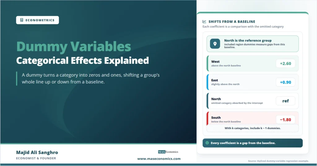
The solution is to include one fewer dummy than there are categories, leaving one category out as the reference, or base, group. With four regions, the model includes three dummies, and the omitted region becomes the baseline against which the other three are measured. The intercept absorbs the reference group, and each included dummy coefficient reports the difference between its category and that reference.

Multiple Categories With a Reference Group

North is the omitted reference region. Each \(\delta\) is the wage gap between its region and the north, at the same level of education.

Reading the Coefficients Against the Baseline

The single most important habit in interpreting dummy variables is to remember what the comparison is against. Every dummy coefficient is read relative to the omitted category, and the choice of which category to omit changes the numbers even though it does not change the underlying relationships. The reference group is the silent term in every comparison.

Table 1. Reading Region Dummies Against the North Baseline

Term	Coefficient	Std. error	Interpretation
Constant \(\beta_0\)	12.40	(0.70)	North wage at zero education (baseline)
Education \(\beta_1\)	2.05***	(0.16)	Return per year, common to all regions
South \(\delta_1\)	-1.80**	(0.60)	South earns 1.80 less than the north
East \(\delta_2\)	0.90	(0.62)	East earns 0.90 more than the north, not significant
West \(\delta_3\)	2.60***	(0.58)	West earns 2.60 more than the north
Implied west wage at zero education	15.00	—	\(\beta_0 + \delta_3 = 12.40 + 2.60\)
Source: Stylized example based on standard formulas. Numbers chosen for illustration.

Read this table correctly and every number is a comparison with the north. The west coefficient of 2.60 does not mean western workers earn 2.60 dollars; it means they earn 2.60 more than otherwise-identical workers in the north. The east coefficient is positive but statistically insignificant, which means the data cannot distinguish eastern wages from northern wages, not that eastern wages are zero. And the negative south coefficient says only that the south sits below the north, not that southern workers earn negative wages. The absolute predicted wage for any region is recovered by adding its dummy coefficient to the constant, as the summary row shows for the west.

Why the Choice of Reference Group Matters for Presentation

Changing the reference group does not change the model. The fitted values, the residuals, and the predicted wage for each region are identical no matter which category is omitted. What changes is the set of comparisons the coefficients report. If the south were chosen as the reference instead of the north, every coefficient would be re-expressed as a gap from the south, and the north, east, and west would all show positive coefficients relative to that lower baseline. The relationships in the data are unchanged; only the vantage point shifts.

This has a practical implication for how results are presented. The reference group should be chosen so that the comparisons readers most want to see are the ones the coefficients display directly. A natural baseline, the largest group, the policy-relevant control condition, or a conventional category that readers expect, makes a table easier to interpret. An arbitrary or tiny reference group forces every comparison to run through a category that may itself be poorly estimated, which inflates standard errors and obscures the contrasts that matter.

Table 2. The Same Data, Two Different Reference Groups

Region	Coefficient vs. north baseline	Coefficient vs. south baseline
North	reference	+1.80
South	-1.80	reference
East	+0.90	+2.70
West	+2.60	+4.40
Wage ranking	Unchanged	Unchanged
Source: Stylized example based on standard formulas. Numbers chosen for illustration.

Both columns describe exactly the same world. The west is always the highest-paid region and the south the lowest, and the spacing between regions is identical. Switching the baseline from north to south simply adds 1.80 to every comparison, because that is the north-south gap that now sits inside the baseline. The lesson is that a dummy coefficient is meaningless without knowing the reference group it is measured against, and that the reference group is a presentation choice rather than a statement about the data.

Letting Slopes Differ, Not Just Intercepts

A dummy on its own shifts the intercept and leaves the slope common to all groups. Sometimes that is the wrong assumption. If the return to education itself differs across regions, a simple dummy cannot capture it, because it forces every region’s wage line to rise at the same rate. Allowing the slope to differ requires multiplying the dummy by the continuous variable, which produces an interaction term. A region dummy interacted with education would let each region have both its own baseline and its own return to schooling, turning parallel lines into lines that fan out.

The distinction is worth keeping clear. A dummy by itself answers the question “does this group sit higher or lower,” while a dummy interacted with a continuous variable answers the further question “does the effect of that continuous variable differ for this group.” The two are often used together, and the move from intercept shifts to slope shifts is the natural next step once categorical baselines are understood. A model that needs different slopes but uses only level dummies will misdescribe the data in the same way a model that omits a needed variable does, by forcing a single relationship onto groups that genuinely differ.

Common Uses Across Applied Economics

Dummy variables appear almost everywhere that data carry structure beyond pure quantities. Seasonal dummies absorb predictable quarterly or monthly patterns in time-series data, separating a genuine trend from regular calendar fluctuation. Fixed-effect dummies for individuals, firms, or countries let a panel model control for unobserved characteristics that stay constant within each unit. A single dummy marking the periods after a policy change is the backbone of before-and-after comparisons, and a dummy that switches on at a known break point is how a model accommodates a structural break in a relationship. In each case the principle is the same: a category becomes a column of zeros and ones, and its coefficient measures a shift relative to the omitted baseline.

The same construction also carries into models where the outcome itself is categorical. When the dependent variable is binary rather than continuous, the regression machinery changes, but explanatory dummies are built and read in the same way, as the treatment of logit and probit models shows. The foundations of fitting and interpreting the underlying line, meanwhile, rest on simple linear regression, with dummies extending that line to as many categorical baselines as the data require.

Explains

Conclusion

The role of dummy variables regression is to bring qualitative, group‑based information into a model designed for numbers by translating each category into a variable that is one when a condition holds and zero otherwise. A single dummy shifts a group’s entire regression line up or down while leaving the slope common to all groups, and its coefficient measures the gap between that group and the category the model leaves out. With more than two categories, the rule is to include one fewer dummy than there are categories and treat the omitted one as the reference, avoiding the perfect collinearity of the dummy variable trap.

Every dummy coefficient is a comparison, never a standalone value, and it is only interpretable in light of the reference group it is measured against. Changing the baseline re‑expresses the comparisons without altering the underlying relationships, which makes the choice of reference group a matter of clear presentation rather than statistical substance. When group differences extend to the slope rather than just the intercept, dummies give way to interaction terms, and when the outcome is itself categorical, the same dummy construction carries into binary‑choice models. Across all of these settings, the discipline is constant: read each dummy as a difference from a baseline, and never lose track of which category that baseline is.

Frequently Asked Questions

Thanks for reading! If you found this helpful, share it with friends and spread the knowledge. Happy learning with MASEconomics