Expansion Path: Cost-Minimizing Input Choices as Output Grows

A bakery producing 500 loaves a day uses a certain mix of ovens and bakers. When demand doubles to 1,000 loaves, the owner does not simply clone the original setup; the new least-cost combination may tilt toward more ovens relative to staff, or the reverse, depending on input prices and the shape of the technology. The expansion path economics describes is the curve that traces this sequence of least-cost input choices as a firm scales output up or down, connecting one cost-minimizing point to the next.

The path is built by repeating a single decision at many output levels. Each level of output has its own isoquant, drawn from the analysis of production functions and isoquant curves, and each isoquant has a cost-minimizing input mix where an isocost line is tangent to it. Joining those tangency points across output levels produces the expansion path, the line that underlies how a firm’s input use and total cost grow with scale, a relationship central to the costs of production.

Connects Successive Tangencies

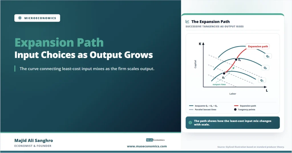
The expansion path is the locus of cost-minimizing input combinations as output varies, holding input prices constant. For each target output, the firm finds the tangency between the relevant isoquant and the lowest isocost line that reaches it. As output rises, the firm needs a higher isoquant, which requires a larger budget and an isocost line farther from the origin. Because input prices are held constant, every one of these isocost lines has the same slope, so they are parallel, and each is tangent to its own isoquant at a distinct point.

The diagram shows three output levels, with Q3 the largest and farthest from the origin. Each isoquant has its own tangency with one of the parallel grey isocost lines, marked by a black dot. The red curve threading through the three tangency points is the expansion path. It records how the cost-minimizing capital-and-labor mix shifts as the firm scales from the smallest output to the largest, and every point on it satisfies the tangency condition for its own output level.

Slope Reflects Constant Input Prices

At every tangency along the path, the same cost-minimizing condition holds: the marginal rate of technical substitution equals the wage-rental ratio. Because input prices stay fixed as output changes, the wage-rental ratio is the same at each output level, so the slope of the isocost line is identical everywhere along the path. This is why the isocost lines are drawn parallel.

Condition Holding Along the Path

The expansion path is the set of input combinations where the marginal rate of technical substitution equals the constant wage-rental ratio, traced as output varies.

The shape of the path then depends on how the technology responds to scale. If the production function is homothetic, the cost-minimizing capital-to-labor ratio stays constant as output grows, and the expansion path is a straight line through the origin. The firm scales both inputs in the same proportion, simply using more of each in a fixed ratio. Homothetic technology, which includes the widely used Cobb-Douglas form, is the case in which scaling up means replicating the same input mix at a larger size.

Shape Records Changing Input Mix

When the technology is not homothetic, the cost-minimizing input ratio changes with output, and the expansion path bends rather than running straight. A path that curves toward the labor axis as output rises means the firm uses proportionally more labor at higher output; a path that curves toward the capital axis means it grows more capital-intensive as it scales. The curvature is a direct record of how the optimal input mix evolves with size.

Table 1. Expansion Path Shape and What It Reveals

Path shape	Input ratio as output rises	Technology type
Straight ray from origin	Constant capital-to-labor ratio	Homothetic, including Cobb-Douglas
Bends toward the labor axis	Rising labor intensity	Non-homothetic, labor-using growth
Bends toward the capital axis	Rising capital intensity	Non-homothetic, capital-using growth
Source: MASEconomics editorial synthesis of standard producer theory.

The straight-line case is the benchmark because it corresponds to the technologies used most often in applied work. A bend away from that benchmark signals that scale itself changes the firm’s optimal reliance on each input, which matters for questions about how employment or capital investment respond as a firm grows.

Generates the Long‑Run Cost Curve

The expansion path is the bridge between input choice and the firm’s cost structure. Each point on the path pairs a level of output with the minimum cost of producing it, since the tangency point is by construction the cheapest way to make that output. Reading the total cost at each output level along the path traces out the firm’s long-run total cost curve directly.

This connection is why the expansion path sits at the center of the transition from production theory to cost theory. The isoquant map describes what is technically possible, the tangency condition selects the cheapest point for each output, and the expansion path collects those points into the sequence that defines how cost grows with scale. Long-run average and marginal cost curves both descend from the total cost curve the path generates.

Assumes Fixed Prices and Free Adjustment

The expansion path holds input prices constant along its entire length. A firm large enough to bid up the wage as it hires more, or to negotiate cheaper capital at volume, faces input prices that change with scale, which tilts the isocost lines at different output levels and distorts the path from the constant-price construction. The standard path is a long-run object in another sense as well: it assumes the firm can freely adjust both capital and labor, which holds in the long run but not in the short run when capital is fixed.

The construction also describes cost-minimizing input choice for each output without specifying which output the firm selects. The level of production depends on demand and the product price, questions outside the path itself. Within these bounds, the expansion path is the precise account of how a cost-minimizing firm changes its input mix as it scales, and it is the structure from which the firm’s long-run cost curves are derived.

Explains

Conclusion

The expansion path economics describes is the curve connecting a firm’s cost-minimizing input combinations across output levels, traced at constant input prices. Each point is a tangency between an isoquant and a parallel isocost line, so the path is the sequence of least-cost choices the firm makes as it scales output up or down. Every point on it satisfies the same condition, that the marginal rate of technical substitution equals the wage-rental ratio.

The shape of the path encodes how the optimal input mix responds to scale. A straight ray from the origin marks homothetic technology, where the capital-to-labor ratio stays constant, and growth means replicating the same mix at a larger size. A path that bends toward one axis marks a technology that grows more intensive in one input as output rises, a departure from the constant-ratio benchmark.

The path’s central role is to generate the firm’s long-run cost curve. Pairing each output level with the minimum cost of its least-cost input bundle traces total cost as a function of output, from which average and marginal cost curves follow. The expansion path is therefore the link that carries the input-choice logic of isoquants and isocosts into the cost theory that governs the firm’s supply behavior.

Frequently Asked Questions

Thanks for reading! If you found this helpful, share it with friends and spread the knowledge. Happy learning with MASEconomics