Understanding the costs of production is essential for firms operating in competitive markets. The ability to efficiently manage both fixed and variable costs helps businesses optimize production, set competitive prices, and allocate resources effectively. The concept of production costs is at the core of economic decision-making, guiding firms in determining how much to produce and at what price to sell their goods or services.
In this article, we provide a comprehensive exploration of short-run and long-run costs, breaking down the different types of production costs and their impact on firm behavior. We also examine how firms achieve profit maximization through careful alignment of marginal cost (MC) and marginal revenue (MR), ensuring sustainable profitability.
Short-Run and Long-Run Cost Dynamics
In microeconomics, firms face different constraints in the short run and the long run. This distinction influences how businesses adjust production levels to remain competitive and efficient.
Short-Run Costs
In the short run, some inputs—such as capital and land—are fixed, limiting a firm’s flexibility. Firms can only adjust variable inputs like labor or raw materials. This creates constraints on production, making it critical for businesses to find the right balance between fixed and variable costs to remain efficient.
Example: A bakery, for instance, can increase or decrease its number of bakers and the amount of flour it buys, but it cannot quickly expand the size of its kitchen or buy new ovens.
The short-run cost structure influences how businesses react to market changes, and firms aim to minimize total costs by managing these variable inputs efficiently.
Long-Run Costs
In the long run, all inputs are variable. Firms have more flexibility to scale operations, add new capital, or adjust labor to meet demand. This period allows businesses to pursue economies of scale—where increased production leads to lower average costs.
Example: The bakery mentioned earlier could, over time, lease a larger space, buy additional ovens, and hire more bakers, thus increasing production capacity.
By varying all inputs, firms in the long run seek to optimize their cost structures and maximize profitability.
This distinction between short-run and long-run decisions is critical because it determines a firm’s ability to adapt to market changes. In the long run, firms aim to minimize costs and achieve optimal efficiency by adjusting all production factors.
Types of Costs
Let’irms must manage several types of costs to remain competitive. Each type plays a unique role in shaping production decisions and influencing profitability.
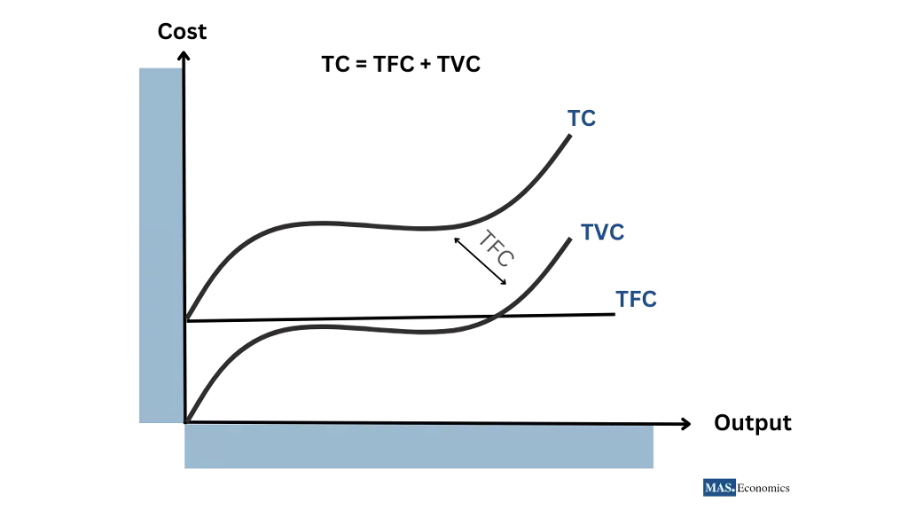
Fixed Costs (FC)
Fixed costs are expenses that do not change with the level of production. Even if a firm produces nothing, it still incurs fixed costs.
Examples: Rent, insurance premiums, and administrative salaries.
Since fixed costs remain constant, firms aim to spread these costs over larger production volumes to reduce the per-unit cost.
Variable Costs (VC)
Variable costs fluctuate with the amount of production. These costs increase as firms produce more units and decrease when production falls.
Examples: Raw materials, hourly wages, and electricity consumption.
The total variable cost (TVC) increases directly to output, influencing the firm’s decision-making regarding production levels.
Total Costs (TC)
The total cost is the sum of fixed and variable costs for a given output level.
Example Calculation:
A bakery with fixed costs of $1,500 and variable costs of $2 per loaf incurs the following total cost for producing 1,000 loaves:
The Law of Diminishing Returns
The law of diminishing returns states that as more units of a variable input (such as labor) are added to fixed inputs (like machinery or land), the additional output generated from each new unit will eventually decrease.
Initially, adding more workers to a production process may increase output significantly. However, as more workers are added, they may become less productive due to limited space or equipment.
Example: In a car assembly plant, hiring more workers initially boosts production, but beyond a certain point, additional workers contribute less to output because of overcrowding on the assembly line.
This principle is particularly relevant in the short run, where fixed resources limit production flexibility. Understanding diminishing returns helps firms determine the optimal number of inputs to avoid inefficiencies.
The table below presents some primary costs a firm faces and indicates whether they are fixed or variable costs:
| Cost Type | Description |
|---|---|
| Fixed Costs (FC) | – Rent (payment for land) – Interest (payment for capital) – Depreciation – Insurance premiums – Property taxes – Administrative costs |
| Variable Costs (VC) | – Wages (payment for labor) – Raw materials – Energy costs – Transportation costs – Marketing costs – Packaging costs |

|
|
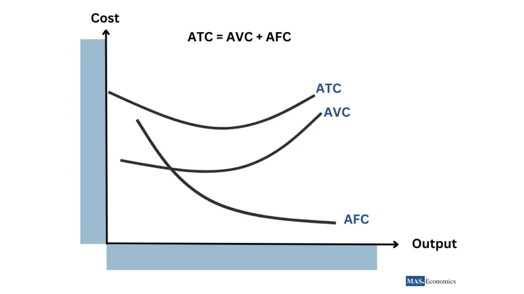
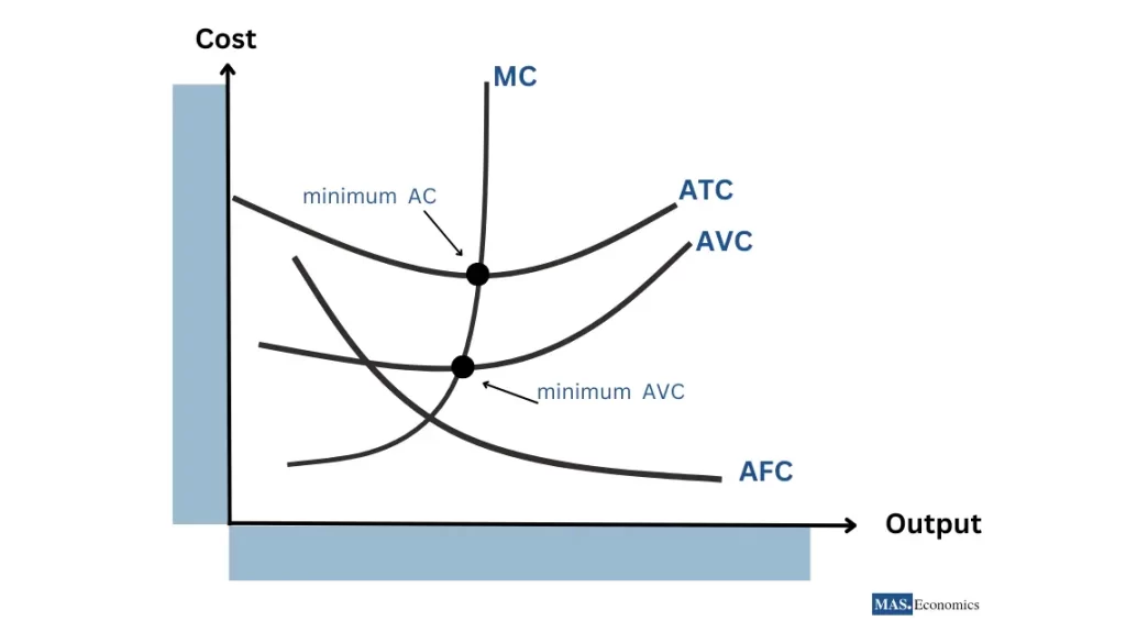
Average Costs: AFC, AVC, and ATC
In microeconomics, firms also analyze per-unit costs to assess production efficiency. These measures include average fixed cost, average variable cost, and average total cost.
Example: A factory with $10,000 in fixed costs producing 1,000 units has:
Average Variable Cost (AVC)
AVC is the variable cost per unit of output.
Example: If the total variable cost for producing 500 units is $2,000, the AVC is:
The AVC curve is typically U-shaped, reflecting economies of scale at low output levels and diminishing returns at higher levels.
Average Total Cost (ATC)
The ATC curve helps firms determine the production level that minimizes per-unit costs.
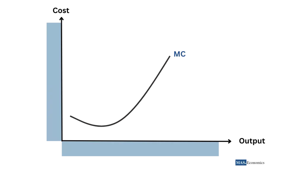
Marginal Cost (MC) and Its Role in Decision-Making
What is Marginal Cost (MC)?
Marginal cost refers to the additional cost incurred by producing one extra unit of output. It is a crucial concept for businesses because it directly impacts profitability. Firms use MC to determine how much to produce: production continues until marginal cost equals marginal revenue (MC = MR), which marks the profit-maximizing level of output.
Where:
- \( \Delta TC \) = Change in total cost
- \( \Delta Q \) = Change in quantity produced (typically one unit)
Example: If producing 100 units cost $5,000, and producing 101 units raises the total cost to $5,050, the marginal cost of the 101st unit is:
Role of MC in Production and Pricing Decisions
Firms produce additional units as long as the marginal cost of producing those units is less than or equal to the marginal revenue (MR) earned from selling them. Once MC exceeds MR, further production results in losses.
Decision Rule:
If MC < MR, increase production.
If MC > MR, decrease production.
If MC = MR, profit is maximized.
MC and the Average Total Cost (ATC) Curve
The MC curve intersects the ATC curve at its minimum point. This point indicates the most efficient production level, where the firm achieves the lowest possible cost per unit. Producing below or beyond this point results in higher average costs.
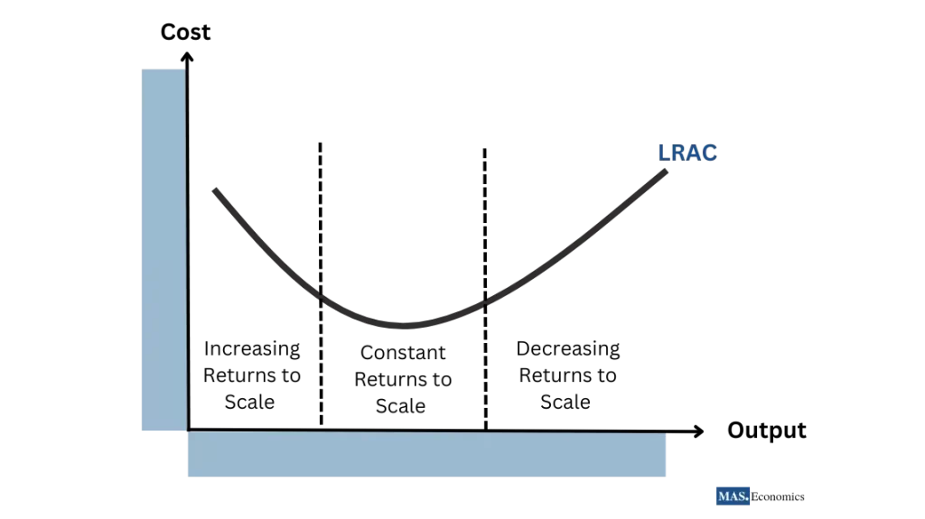
Long-Run Costs and Returns to Scale
Understanding Long-Run Costs
In the long run, all inputs (capital, labor, land) are variable, giving firms the flexibility to adjust their production scale. The long-run cost structure focuses on how average costs change as production scales up or down.
Increasing Returns to Scale:
Output increases more than the proportional increase in inputs, reducing average costs.
Constant Returns to Scale:
Output increases proportionally with inputs, leaving average costs unchanged.
Decreasing Returns to Scale:
Output increases less than input, increasing average costs.
Firms strive to operate at the point where average costs are minimized, known as the minimum efficient scale.
Sunk Costs and Rational Decision-Making
A sunk cost is a cost that has already been incurred and cannot be recovered. Rational decision-making requires firms to ignore sunk costs when making future decisions.
Example: A pharmaceutical company invests heavily in research but discovers the drug won’t be profitable. Ignoring sunk costs, the firm should stop further investment and focus on more viable projects.
Revenue Analysis
Total Revenue (TR)
Revenue is the income generated from selling goods or services. Firms analyze revenue to determine how much to produce and at what price.
Where:
- \( P \) = Price per unit
- \( Q \) = Quantity sold
Example: If a firm sells 100 units at $10 each, the total revenue is:
Marginal Revenue (MR)
Marginal revenue measures the additional income earned from selling one more unit of a good or service.
Where:
- \( \Delta TR \) = Change in total revenue
- \( \Delta Q \) = Change in quantity sold (typically 1 unit)
Example: If selling the 101st unit raises total revenue from $1,000 to $1,100, the MR for the 101st unit is:
Average Revenue (AR)
Average revenue is the revenue earned per unit sold:
Example: If total revenue is $500 from selling 50 units, the AR is:
In a perfectly competitive market, AR equals price since all units are sold at the same price. In imperfect competition, AR decreases as the firm lowers prices to sell more units.
Profit Maximization: Where MC = MR
Firms maximize profits by producing at the point where marginal cost equals marginal revenue (MC = MR). Producing beyond this point results in losses while producing less means the firm is not fully exploiting its profit potential.
In perfectly competitive markets, profit maximization occurs where MC = P, as the firm has no control over prices. In monopolistic or imperfect markets, the condition becomes MC = MR, where the marginal revenue curve slopes downward because firms must lower prices to sell additional units.
Firms that operate at the optimal production level—where MC intersects MR—achieve the highest possible profit. Producing beyond this point raises costs more than revenues while producing less underutilizes available capacity and misses profit opportunities.
The Profit-Maximization Rule
Firms aim to maximize profit by producing where marginal cost (MC) equals marginal revenue (MR).
If MC < MR: Increase production.
If MC > MR: Decrease production.
If MC = MR: Profit is maximized.
Mathematical Example of Profit Maximization
Assume the following functions:
Taking derivatives to find MR and MC:
Setting \( MR = MC \):
The profit-maximizing output is 15 units.
Normal Profit and Economic Profit
To stay in business in the long run, firms must earn at least normal profit, which covers both explicit and implicit costs, including opportunity costs. Normal profit ensures the firm remains sustainable without attracting or deterring new competitors.
- Normal Profit: The minimum profit required to keep a firm in operation.
- Economic Profit: Profit above normal profit, which attracts competitors into the market.
| Feature | Normal Profit | Economic Profit |
|---|---|---|
| Definition | The minimum profit that a firm needs to make in order to stay in business in the long run. | The profit that a firm makes above and beyond normal profit. |
| How it is calculated | Total revenue – Total cost | Total revenue – Total cost – Normal profit |
| Occurs in | Perfectly competitive markets | Imperfectly competitive markets |
| Attracts firms | No | Yes |
|
|
||
Conclusion
Understanding the costs of production is essential for firms seeking to optimize production and maximize profits. Firms use concepts like MC, ATC, and MR to align production with profitability. Efficient management of costs in both the short run and long run allows firms to remain competitive while pursuing economies of scale. By following rational decision-making principles, businesses can ensure long-term growth and success.
FAQs:
What are short-run and long-run costs in microeconomics?
Short-run costs involve fixed inputs like capital, limiting flexibility, while firms can adjust variable inputs like labor. Long-run costs allow firms to vary all inputs, enabling them to scale operations and achieve efficiency through economies of scale.
What is the difference between fixed and variable costs?
Fixed costs remain constant regardless of production levels, such as rent or insurance, while variable costs, like raw materials, fluctuate with the level of output.
What is the law of diminishing returns?
The law of diminishing returns states that adding more units of a variable input to fixed inputs will eventually yield lower additional output, impacting efficiency in the short run.
How do marginal cost (MC) and marginal revenue (MR) guide production decisions?
Firms maximize profit by producing where MC equals MR. If MC is lower than MR, production increases, while if MC exceeds MR, firms reduce output to avoid losses.
What are economies of scale, and why are they important?
Economies of scale occur when increasing production reduces average costs due to factors like bulk purchasing or labor specialization, helping firms remain competitive.
What is the role of sunk costs in decision-making?
Sunk costs are past expenses that cannot be recovered. Rational firms ignore sunk costs and focus on future decisions that maximize profitability.
How do firms determine optimal production levels?
The optimal production level is where MC equals MR, ensuring that the additional cost of producing one more unit matches the revenue it generates, maximizing profit.
What is the difference between normal profit and economic profit?
Normal profit covers all costs, including opportunity costs, ensuring sustainability. Economic profit exceeds normal profit and attracts new market entrants.
Why is average cost analysis important for businesses?
Average cost analysis helps firms find the production level that minimizes per-unit costs, ensuring efficient operations and competitive pricing.
How do short-run and long-run costs influence profitability?
In the short run, firms adjust variable inputs to manage costs, while in the long run, they optimize all inputs to achieve economies of scale and sustain long-term profitability.
Thanks for reading! Share this with friends and spread the knowledge if you found it helpful.
Happy learning with MASEconomics