Hicksian vs Marshallian demand answers a deceptively simple question two different ways: how much of a good will a consumer buy when its price changes? Marshall built his curve in 1890 by holding nominal income fixed and tracing observed purchases. Hicks built his in 1939 by holding utility fixed and asking how much would be purchased if the consumer were compensated for the price change. The two curves coincide at one point, diverge everywhere else, and the gap between them is the foundation of modern welfare economics.
Both curves emerge from the same underlying preferences, the same budget constraint, and the same indifference map. They differ in one variable: what is held constant as the price moves. That single methodological choice produces curves with different slopes, different elasticities, and different uses in applied work. Anyone who has worked with indifference curves and consumer choice has implicitly drawn both of them without naming the distinction. This article names it, formalises it, and shows why empirical economists almost always estimate one while welfare economists almost always need the other.
The Dual Consumer Problem
Marshallian demand comes from the utility maximisation problem. The consumer faces prices \( p_1, p_2 \) and income \( m \), and chooses bundle \( (x_1, x_2) \) to maximise utility \( u(x_1, x_2) \) subject to \( p_1 x_1 + p_2 x_2 \leq m \). The solution gives Marshallian demand \( x_i^M(p_1, p_2, m) \), a function of prices and income. This is what consumers actually do in markets, and it is what survey data and scanner data measure.
Hicksian demand comes from the expenditure minimisation problem. The consumer is asked to reach a fixed utility level \( \bar{u} \) at the lowest possible cost. Formally, minimise \( p_1 x_1 + p_2 x_2 \) subject to \( u(x_1, x_2) \geq \bar{u} \). The solution gives Hicksian demand \( x_i^H(p_1, p_2, \bar{u}) \), a function of prices and the target utility. This is a hypothetical construct: in the real world, consumers do not minimise expenditure at a fixed utility level. They maximise utility at a fixed income. But the mathematical mirror image is what makes welfare analysis tractable.
The two problems are dual to each other. Mas-Colell, Whinston, and Green develop the duality formally in Chapter 3 of Microeconomic Theory, showing that the same preference structure can be recovered from either program. At the consumer’s optimal point, with income \( m \) just sufficient to reach utility \( \bar{u} \), the two demands agree:
where \( e(p, \bar{u}) \) is the expenditure function, the minimum money required to reach \( \bar{u} \) at prices \( p \). Move away from that point, and the demands diverge, because the two programs hold different things constant.
What Hicksian and Marshallian Demand Hold Constant
This is the heart of the distinction. When the price of good 1 falls, the Marshallian consumer keeps the same nominal income, becomes richer in real terms, and adjusts purchases accordingly. The Hicksian consumer, in contrast, is hypothetically compensated so that the original utility level remains attainable. The Hicksian curve traces only the response to the relative price change, with all income effect stripped out.
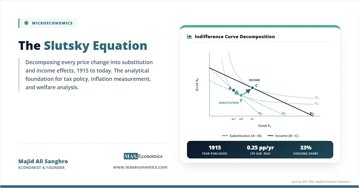
Sir John Hicks introduced this construction in Value and Capital (1939), building on Eugen Slutsky’s 1915 algebraic decomposition. Hicks framed it as a way to ask what the consumer would buy if the real income gain from a price cut were taken back through a lump-sum tax that exactly restored the old utility. The thought experiment is artificial, but it isolates the substitution effect cleanly. The Marshallian response, by contrast, blends the substitution effect and the income effect into a single observed change, which is exactly what makes the Marshallian curve easy to estimate from market data and hard to use for welfare measurement.
The relationship between the two is captured by the Slutsky equation, the bridge that connects them:
Read it left to right. The total Marshallian response to a price change equals the pure Hicksian substitution response minus an income effect. The size of the income effect is the product of how much of good \( j \) the consumer was already buying and how strongly demand for good \( i \) responds to changes in income. For a deeper graphical and algebraic treatment of how this equation is derived, our walkthrough of the Slutsky decomposition takes the same diagram apart line by line.
Comparing the Two Demand Functions
The five rows below are the operational distinctions a graduate student or applied economist needs to keep straight when moving between estimation and welfare work.
| Feature | Marshallian (Uncompensated) | Hicksian (Compensated) |
|---|---|---|
| Mathematical definition | \( x_i^M(p, m) = \arg\max u(x) \text{ s.t. } p \cdot x \leq m \) | \( x_i^H(p, \bar{u}) = \arg\min p \cdot x \text{ s.t. } u(x) \geq \bar{u} \) |
| What is held constant | Nominal income \( m \) | Utility level \( \bar{u} \) |
| Slope properties | Almost always negative; can slope upward for Giffen goods because the income effect dominates substitution | Always negative for normal substitution behaviour; \( \partial x_i^H / \partial p_i \leq 0 \) is guaranteed by concavity of the expenditure function |
| Components of price response | Substitution effect plus income effect (the total observed change) | Substitution effect only (income effect removed by compensation) |
| Primary use | Empirical demand estimation; market-level forecasting; tax incidence studies using observed quantities | Welfare measurement through compensating and equivalent variation; deadweight loss calculations; Shephard’s lemma |

|
||
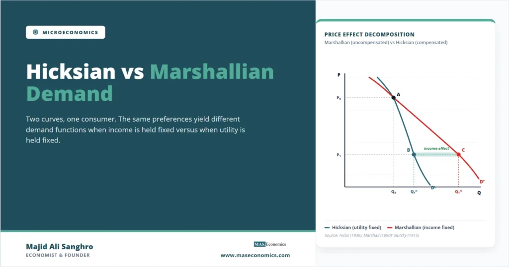
The table fixes the algebra; the diagram fixes the geometry.
Three features of the diagram repay careful reading. First, the two curves intersect at point A, the initial equilibrium. At that price, nominal income exactly buys the bundle that delivers utility \( \bar{u} \), so the utility-maximising and expenditure-minimising consumer makes identical choices. Second, when the price falls from \( P_0 \) to \( P_1 \), the Hicksian consumer moves only to point B because the compensation has been taken back. The Marshallian consumer moves all the way to point C, because nominal income now buys more in real terms. The horizontal distance B to C is the income effect on the quantity demanded of good 1. Third, the Marshallian curve is flatter than the Hicksian curve below the initial price for a normal good. The income effect reinforces the substitution effect, so a given price cut elicits a larger Marshallian response than a Hicksian response.
For an inferior good, the picture inverts: the income effect partially cancels the substitution effect, the Marshallian curve is steeper than the Hicksian curve, and in the extreme case of a Giffen good, the income effect dominates and the Marshallian curve slopes upward while the Hicksian curve continues to slope down. The Hicksian curve, in other words, isolates what the substitution effect can produce on its own.
MASEconomics Explains
Two demand curves, two questions answered
These concepts are explored in depth across our educational articles library.
Explore the MASEconomics BlogHicksian Demand in Welfare Measurement
The use cases divide cleanly. Empirical economists who estimate price elasticities from supermarket scanner data, transportation surveys, or tax-reform experiments are recovering Marshallian elasticities, because the observed quantities respond to both substitution and income effects together. Marshall’s Principles of Economics (1890) introduced demand schedules precisely as a tool for reading market behaviour, and the modern estimation toolkit still treats market-observed demand as the Marshallian object.
Welfare measurement is a different problem. When a price changes, the welfare loss to the consumer is the area to the left of the demand curve between the old and new prices, but only if that area corresponds to a meaningful money equivalent of the utility change. The Marshallian demand curve does not deliver that money equivalent in general, because the consumer’s marginal utility of income changes as real income changes along the curve. Robert Willig showed in a classic 1976 American Economic Review note that the Marshallian consumer-surplus approximation can be acceptable when income effects are small, but it is an approximation, not an exact welfare measure.
The Hicksian demand curve fixes utility, so the area to its left between two prices is an exact money measure of the utility change. Two related Hicksian measures are used in practice. Compensating variation asks how much money must be taken away after a price cut to leave the consumer indifferent to the original situation. Equivalent variation asks how much money must be given to the consumer instead of the price cut to deliver the same utility gain. Both quantities are recovered from the expenditure function and the Hicksian demand curve. They are the standard inputs to deadweight-loss calculations in public economics and to cost-benefit analysis of policy changes. Hicks’s original justification for building the compensated curve was exactly this welfare problem.
Slutsky Sign Restrictions
The Slutsky equation has direct empirical content. The own-price Hicksian substitution effect must be non-positive: a consumer who is compensated for a price increase cannot consume more of the now-more-expensive good without violating expenditure minimisation. This is the law of compensated demand, and it is the only universal sign restriction in consumer theory. The Marshallian own-price response carries no such guarantee. If good \( i \) is inferior and accounts for a large share of the budget, the income effect can swamp the substitution effect and produce upward-sloping Marshallian demand.
This is why Giffen goods are theoretically possible but empirically rare. The conditions require a strongly inferior good that absorbs a large share of expenditure, a configuration that holds for staples in low-income populations and almost nowhere else. The Hicksian demand curve, in contrast, is always downward-sloping by construction. If empirical work appears to find positive own-price slopes in the substitution matrix, the diagnosis is almost always that the income effect has been imperfectly netted out, not that compensated demand has misbehaved. This empirical content reaches back to revealed preference theory, where the Weak and Strong Axioms guarantee precisely the negative semi-definiteness of the Slutsky substitution matrix.
Cross-price effects extend the same logic. Hicksian cross-price effects are symmetric: \( \partial x_i^H / \partial p_j = \partial x_j^H / \partial p_i \). This follows from the symmetry of the second partial derivatives of the expenditure function. Marshallian cross-price effects are not symmetric in general because the income terms in the Slutsky equation differ across goods. Testing for symmetry in empirical demand systems is therefore a test of theoretical consistency, not of the model’s predictions about consumer behaviour.
Deriving Demand via Roy and Shephard
The two demand functions are reachable from the dual representations of the consumer problem through two parallel results. Roy’s identity recovers Marshallian demand from the indirect utility function \( v(p, m) \):
Shephard’s lemma recovers Hicksian demand from the expenditure function \( e(p, \bar{u}) \):
Shephard’s lemma is exact: the partial derivative of the expenditure function with respect to a price is the Hicksian demand for that good, evaluated at the same utility level. The result follows from the envelope theorem applied to the expenditure-minimisation program. Roy’s identity, despite its more complex form, has the same logical status for the utility-maximisation program. Together, they explain why graduate textbooks treat the expenditure function and indirect utility function as the primary objects of consumer theory: once either is known, the corresponding demand function and its dual partner are both two steps away.
The duality has a satisfying consistency check. Substituting \( m = e(p, \bar{u}) \) into Marshallian demand recovers Hicksian demand, and substituting \( \bar{u} = v(p, m) \) into Hicksian demand recovers Marshallian demand. The consumer’s problem can be entered through either door, and the same underlying preferences are mapped out. The choice of door is dictated by what is observable. Income is observable, so applied work starts with the utility-maximisation program. Utility is not observable, so welfare work moves to the expenditure-minimisation dual where compensating quantities can be priced.
When the Distinction Disappears
Two cases collapse the distinction between the two curves, and recognising them clarifies when the choice between Hicks and Marshall actually matters in practice.
The first case is quasilinear preferences. If utility takes the form \( u(x_1, x_2) = x_1 + g(x_2) \), where good 1 enters linearly, then the income effect on good 2 is zero. Demand for good 2 depends only on its own price, not on income, and the Marshallian and Hicksian curves for good 2 coincide everywhere. Consumer surplus computed from the Marshallian curve becomes an exact welfare measure. This is why undergraduate textbooks often use quasilinear examples when teaching consumer surplus: the distinction does not bite, so a single curve suffices. Hal Varian’s Intermediate Microeconomics develops the quasilinear case carefully.
The second case is small-budget shares. When the good in question is a tiny fraction of total expenditure, the income effect of a price change for that good is negligible. Demand for a single brand of breakfast cereal, for example, responds almost entirely through substitution; the income effect of doubling the cereal price barely registers in a household’s overall budget. For this reason, the gap between Marshallian and Hicksian elasticities of disaggregated goods is usually small, and applied price-elasticity estimates from market data can be used in welfare exercises with limited bias. The Willig bounds quantify how small the bias is as a function of the budget share and the income elasticity.
The cases where the distinction matters most are large-budget-share goods (housing, food at low incomes, energy in countries where it is heavily subsidised) and large price changes. In these settings, the income effect is substantial, and the Marshallian curve diverges meaningfully from the Hicksian. Tax incidence and welfare analysis of major reforms must use the compensated curve to avoid systematic bias in deadweight-loss estimates. Our overview of welfare economics and Pareto efficiency traces this welfare apparatus from the compensated curve to the social welfare function.
The Joint Interpretation of Both Curves
The dual structure of consumer theory is not a mathematical decoration. It is the device that lets economists separate two intertwined effects of a price change and assign each to the right tool. The Marshallian curve records what the consumer does; the Hicksian curve records what the price change would do if real income were held still. The Slutsky equation translates between them. Holding the preference structure fixed, the two curves are different shadows of the same object, cast under different lighting.
The methodological lesson generalises. Whenever an applied result depends on a price change, it is worth asking whether the response of interest is the total behavioural response (Marshallian) or the substitution response with income removed (Hicksian). Tax-elasticity estimates used in revenue forecasts need the Marshallian response. Deadweight-loss estimates used in cost-benefit analysis need the Hicksian. Confusing the two is a frequent source of disagreement in policy debates, especially when the same numerical elasticity is invoked in both contexts. The convexity and monotonicity assumptions that make the consumer problem well-posed, examined in monotonicity, convexity, and differentiability of preferences, are precisely the assumptions that make both curves well-defined and the Slutsky equation valid.
Conclusion
Hicksian vs Marshallian demand is the central duality of consumer theory and the operational distinction between empirical demand estimation and welfare measurement. Marshallian demand records the consumer’s response at constant nominal income, blending substitution and income effects in a single observable change. Hicksian demand records the response at constant utility, isolating the substitution effect through hypothetical compensation. The two curves intersect at the initial equilibrium, diverge as the price moves, and are connected by the Slutsky equation. Marshallian demand drives forecasting and elasticity estimation. Hicksian demand drives compensating and equivalent variation, deadweight-loss calculations, and the welfare side of public economics. The choice between them is dictated by the question, not by preference.
Frequently Asked Questions
What is the difference between Hicksian and Marshallian demand?
Marshallian demand holds nominal income constant and combines the substitution and income effects of a price change. Hicksian demand holds utility constant by hypothetically compensating the consumer for price changes, capturing only the substitution effect. The two functions agree at the initial equilibrium but diverge as prices move, and they are linked by the Slutsky equation.
Why is the Hicksian demand curve always downward sloping?
Hicksian demand comes from expenditure minimisation at a fixed utility level. The expenditure function is concave in prices, which mathematically implies that its second derivative with respect to own price is non-positive. By Shephard’s lemma, this second derivative is the slope of Hicksian demand, so own-price Hicksian responses are always non-positive. This is the law of compensated demand and is the only universal sign restriction in consumer theory.
Which demand curve is used in welfare economics?
Welfare economics primarily uses Hicksian demand because the area to the left of the Hicksian curve between two prices is an exact money measure of the utility change. This area defines compensating variation and equivalent variation, the standard welfare measures for price changes. Marshallian consumer surplus is an approximation that is accurate only when income effects are small, as Willig (1976) formally showed.
Are Hicksian and Marshallian demand the same for Giffen goods?
No. For a Giffen good, the Marshallian demand curve slopes upward over some price range because the negative income effect on a strongly inferior good outweighs the negative substitution effect. The Hicksian demand curve still slopes downward because compensation removes the income effect entirely. Giffen behaviour is a Marshallian phenomenon that disappears under Hicksian compensation.
How do you derive Hicksian demand from Marshallian demand?
The Slutsky equation links the two: the Hicksian price derivative equals the Marshallian price derivative plus the quantity demanded times the Marshallian income derivative. Alternatively, substitute the expenditure function \( m = e(p, \bar{u}) \) into Marshallian demand to obtain Hicksian demand: \( x^H(p, \bar{u}) = x^M(p, e(p, \bar{u})) \). Both routes rely on the duality between utility maximisation and expenditure minimisation developed in Mas-Colell, Whinston, and Green (1995).
Thanks for reading! If you found this helpful, share it with friends and spread the knowledge. Happy learning with MASEconomics