Welcome to MASEconomics, your guide to the world of economics. In this blog, we will explore consumer behavior, a pivotal field in economics that helps us understand how individuals make choices within the constraints of limited resources. Central to this field is the concept of indifference curves, which visually represent a consumer’s preferences for different combinations of goods that provide the same level of satisfaction or utility.
Before we delve into indifference curves, it’s essential to grasp how utility is measured. There are two fundamental approaches: cardinal and ordinal utility.
- Cardinal Utility: In this approach, satisfaction is quantified using numerical values. It allows for precise comparisons of satisfaction between different goods.
- Ordinal Utility: This method ranks preferences without assigning specific numerical values. It provides qualitative insights into consumer choices.
For our exploration, we’ll predominantly focus on ordinal utility, as it is more commonly used in economics.
Now that we have a basic understanding of utility, let’s look closer at indifference curves and their role in consumer behavior.
Indifference Curves
Indifference curves serve as the cornerstone of understanding consumer behavior. These graphical representations portray a consumer’s preferences for two goods, revealing all combinations of these goods that provide the same level of satisfaction.
Indifference schedule
To provide a more detailed view of indifference curves, an indifference schedule comes into play. It’s essentially a table that lists combinations of two goods, each offering the same level of satisfaction. This table complements our visual understanding of indifference curves.
Graph 1: Indifference Curve with Indifference Schedule
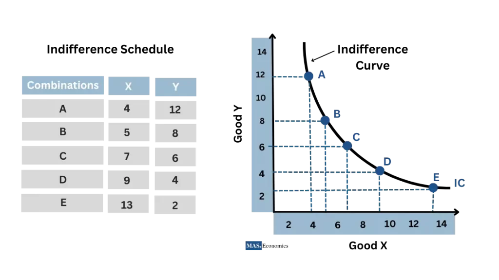
In this graph, we see how different combinations of two goods (e.g., apples and oranges) form points along the indifference curve, where each point represents the same level of satisfaction. This curve is constructed using the indifference schedule, providing a foundation for understanding how consumers make choices between different goods.
Indifference map
Indifference maps enhance our understanding of consumer preferences by incorporating multiple indifference curves. These maps offer a visual summary of a consumer’s choices, showcasing how their preferences evolve as they move along different curves. Here’s an example of what an indifference map may look like:
Graph 2: Indifference Map
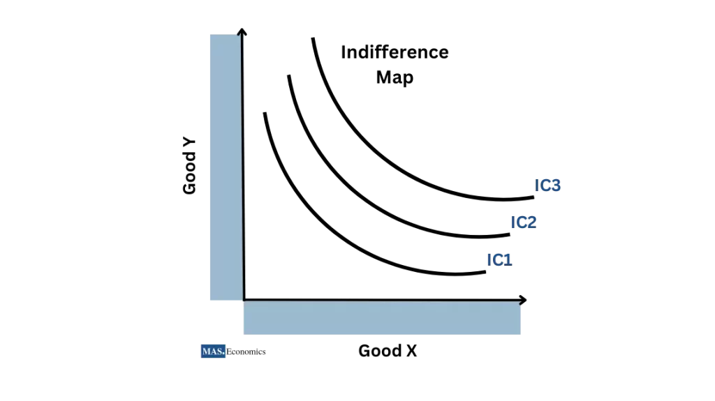
The graph shows several indifference curves, each representing a different satisfaction level. As consumers move to higher curves, their utility increases, showing a preference for those combinations of goods. The map helps visualize how different bundles of goods provide varying levels of satisfaction.
Assumptions Behind Indifference Curves
Indifference curves rest on several assumptions:
- Completeness: Consumers can rank all possible combinations of goods in terms of utility.
- Transitivity: If a consumer prefers combination A to B and combination B to C, then the consumer prefers A to C. This ensures consistency in consumer preferences.
- Non-satiation: Consumers always desire more of both goods, indicating that they are never fully satisfied.
Marginal Rate of Substitution (MRS)
The MRS quantifies how much of one good a consumer is willing to give up for an additional unit of another good without changing their satisfaction level. It can be constant or diminishing along an indifference curve.
- MRS constant: The MRS is constant when the consumer is indifferent between all the combinations of goods on an indifference curve. This means that the consumer is willing to give up the same amount of one good in exchange for the same amount of the other good, no matter where they are on the indifference curve.
- MRS diminishing: The MRS is diminishing when the consumer moves down an indifference curve. This means that the consumer becomes less willing to give up one good in exchange for another as they consume more of the first good.
The properties of indifference curves
| Property | Description |
|---|---|
| Downward-sloping | Consumers prefer more of both goods to less of both goods. |
| Not straight lines | Consumers are willing to trade off one good for another. The more steeply an indifference curve slopes, the less willing the consumer is to trade off one good for another. |
| Do not intersect | Consumers cannot be indifferent between two different combinations of goods. |
| Higher indifference curves represent higher levels of utility | A consumer prefers to be on a higher indifference curve than a lower one. |
Types of Indifference Curves
Indifference curves come in various shapes, reflecting diverse consumer preferences:
- Convex Indifference Curves: These curves signify that consumers are willing to trade one good for another, but only up to a point. The steepness of the curve indicates the willingness to trade.
- Parallel Indifference Curves: Parallel curves denote perfect substitutes, where consumers are indifferent to any combination as long as the total quantity remains the same.
- Complementary Indifference Curves: These curves indicate perfect complements, where consumers only want to consume the two goods together in specific proportions.
Budget Line
The budget line, represented as a straight line in a graph, is a pivotal concept. It delineates the combinations of goods a consumer can afford, given their income and the prices of goods. Let’s visualize it to understand better:
Graph 3: Budget Line
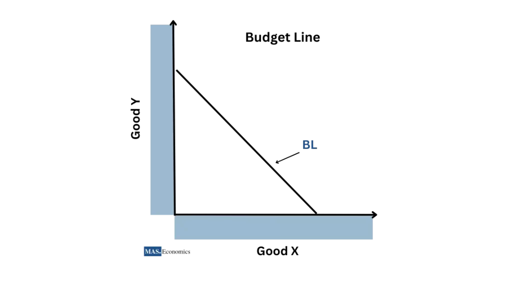
The budget line reflects the trade-offs consumers must make between two goods based on their income. If the price of a good changes, or if the consumer’s income changes, the slope of the budget line will adjust, affecting their choices. The line represents the maximum combinations of goods a consumer can purchase.
Changes in the Budget Line
When a consumer’s income or the price of goods changes, the budget line shifts. This shift illustrates how consumption choices adapt to new financial constraints or opportunities.
Graph 4: Impact of Income and Price Changes on Budget Line
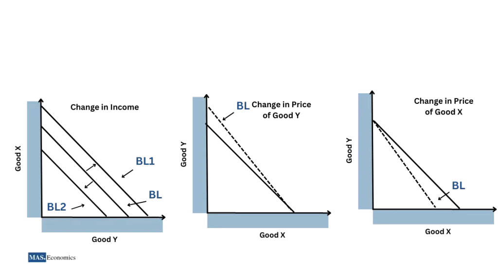
When income increases, the budget line shifts outward, allowing consumers to purchase more of both goods. Conversely, a price increase in one good makes the line steeper, reducing the consumer’s ability to purchase that good.
The implications of the budget line
The budget line has several implications for understanding consumer choices. First, it shows that consumers are limited by their income and the prices of goods. This means consumers cannot afford to buy any combination of goods they want.
Second, it shows that consumers must choose how to allocate their limited resources. This means that consumers must decide which goods they want to buy and how much of each good they want to buy.
Third, it shows that the opportunity cost of a good increase as the consumer consumes more of that good. This is because the consumer has to give up more and more of other goods to obtain each additional unit of the good.
Consumer Equilibrium
Consumer equilibrium is the sweet spot where a consumer’s preferences align harmoniously with their budget constraints. It represents the point where a consumer attains the highest level of satisfaction within their financial boundaries. Understanding this equilibrium is crucial in comprehending real-world consumer choices.
Graph 5: Consumer Equilibrium
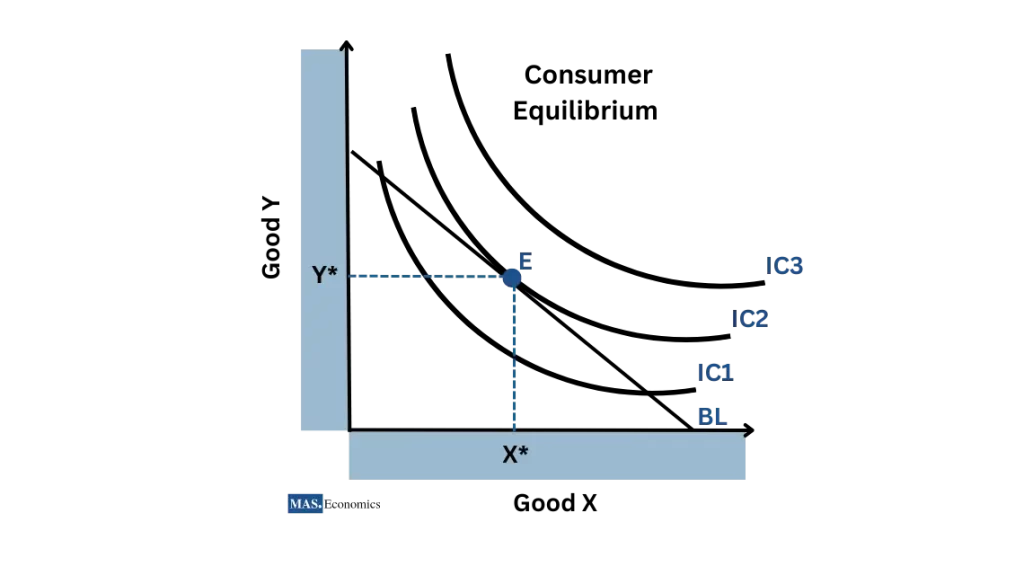
In this graph, consumer equilibrium occurs where the budget line is tangent to the highest indifference curve. At this point, the consumer maximizes their satisfaction given their budget, choosing a combination of goods that aligns with their preferences and financial capacity.
The dynamic nature of consumer equilibrium
Consumer equilibrium isn’t stagnant; it adapts to changing circumstances. For instance, an increase in income shifts the budget line outward, expanding consumption possibilities.
| Factor | Effect on budget line | Effect on indifference curves | Effect on consumer equilibrium |
|---|---|---|---|
| Price of a good decreases | Shifts outward | Does not shift | Consumer moves to a new equilibrium point, consuming more of the good |
| Consumer’s income increases | Shifts outward | Does not shift | Consumer moves to a new equilibrium point, consuming more of all goods |
| Consumer’s preferences change | Does not shift | Shifts | Consumer moves to a new equilibrium point, consuming different quantities of goods |
Income Effect and Income Consumption Curve
The income effect explores how changes in a consumer’s income affect their consumption choices while keeping prices constant. When a consumer’s income increases, they can afford more of both goods, shifting their consumption patterns.
Graph 6: Income Consumption Curve
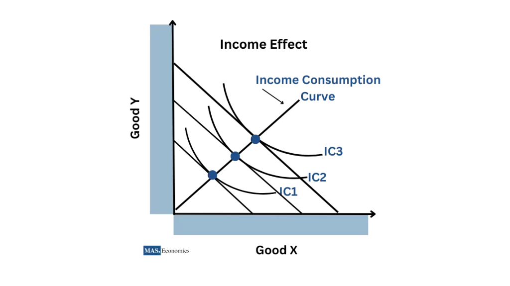
In this graph, as income increases from a lower level (IC1) to a higher level (IC3), the consumption of both goods increases, moving the equilibrium point further out. The Income Consumption Curve (ICC) traces the path of equilibrium points as the consumer’s income rises, showing their increased purchasing power.
Graph 7: Income Effect with Inferior Goods
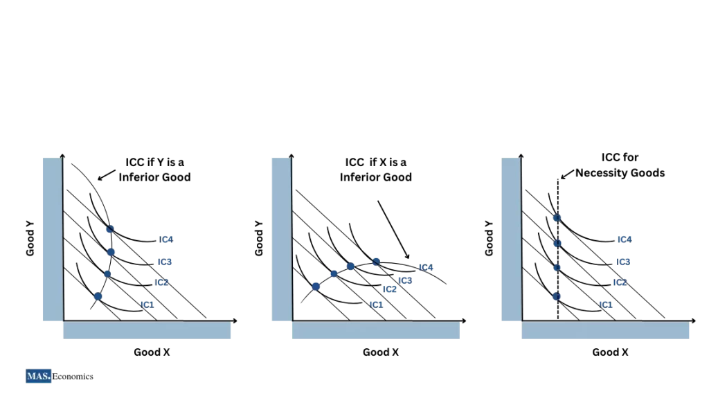
Unlike normal goods, the demand for inferior goods decreases as income increases. In this graph, as the consumer’s income rises, they shift their consumption away from the inferior good towards a more preferred good, resulting in a backward-bending ICC for the inferior good.
Price Effect: The Influence of Price Changes
Price fluctuations also significantly affect consumption behavior. When the price of a good drops, consumers can afford more of it, leading to increased consumption. This phenomenon is encapsulated in the Price Consumption Curve (PCC). Observe how price changes affect consumption:
Graph 7: Price Consumption Curve
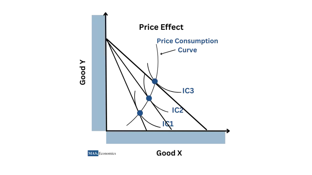
As the price of a good decreases, the PCC shifts, reflecting an increase in consumption of the cheaper good while maintaining satisfaction levels.
Substitution Effect: Swapping Goods
The substitution effect is a key driver of consumer choices. It emerges when consumers substitute cheaper goods for more expensive ones as prices change. This effect is crucial in understanding how consumers respond to price variations. Visualize this substitution process to grasp its significance:
Graph 8: Substitution Effect on Indifference Curve
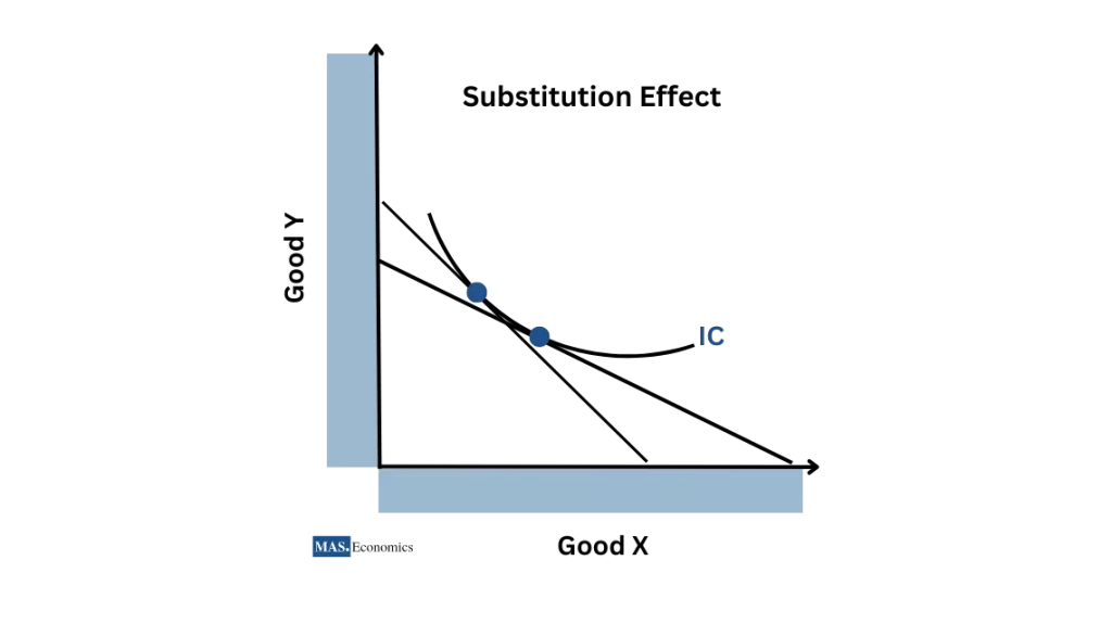
This graph highlights how consumers adjust their consumption between two goods when the price of one decreases, making the cheaper good more attractive.
Bringing it All Together
Consumer choices are shaped by the interplay of income, price, and substitution effects. The outcome depends on various factors, including consumer preferences and the relative strengths of these effects. Let’s consolidate our understanding of these interactions.
| Effect | Description |
|---|---|
| Income effect | The change in consumption that results from a change in income, holding prices constant. |
| Price effect | The change in consumption that results from a change in price, holding income constant. |
| Substitution effect | The change in consumption that results from a change in price, holding income constant. |
The interplay of these effects can be complex and depends on several factors, including the consumer’s preferences, the prices of the goods, and the consumer’s income.
The Cardinal Utility Approach
While ordinal utility theory helps us understand preferences, cardinal utility theory quantifies satisfaction. It assigns numerical values to utility, facilitating direct comparisons of satisfaction between goods. This approach is essential for a deeper understanding of consumer behavior.
Total Utility and Marginal Utility
Total utility represents the overall satisfaction derived from consuming a good, while marginal utility measures the additional satisfaction gained from consuming one more unit. The law of diminishing marginal utility stipulates that as more of a good is consumed, each additional unit provides diminishing satisfaction. Visualize this concept for a clearer grasp: [Add Total and Marginal Utility graph here]
Law of Equi-Marginal Utility
The law of equi-marginal utility offers valuable insights into consumer choices. It suggests that consumers maximize satisfaction when the marginal utilities of all goods they consume are equal. This principle guides rational consumer behavior.
Conclusion
Understanding consumer behavior requires analyzing indifference curves, budget lines, and utility theory. These concepts explain how consumers make choices within their financial limits and preferences. They provide a structured approach to examining decisions in the face of limited resources and varying economic conditions.
FAQs
What is the significance of indifference curves in economics?
Indifference curves help illustrate consumer preferences, showing combinations of goods that offer the same level of satisfaction. They are crucial for analyzing consumer choice behavior and understanding trade-offs between goods.
How does the marginal rate of substitution (MRS) affect consumer choices?
The MRS reflects a consumer’s willingness to trade one good for another while maintaining the same satisfaction level. It influences the shape of indifference curves and the decisions consumers make as they balance their preferences.
What role does the budget line play in consumer equilibrium?
The budget line represents the combinations of goods a consumer can afford given their income and prices. It intersects with indifference curves to determine the optimal consumption point, where satisfaction is maximized within the consumer’s budget.
How do income and price changes impact consumer behavior?
Income changes shift the budget line outward or inward, influencing how much consumers can afford. Price changes alter the slope of the budget line, impacting the quantity of each good a consumer can purchase and leading to substitution or income effects.
What is the difference between the income effect and the substitution effect?
The income effect refers to changes in consumption resulting from a change in purchasing power, while the substitution effect involves consumers opting for cheaper alternatives when relative prices change.
Thanks for reading! If you enjoyed this series, spread the knowledge by sharing it with friends and on social media.
Happy learning with MASEconomics!