An equilibrium equation can determine price, output, or interest rates even when it cannot be solved neatly into an explicit formula. Implicit function theorem economics explains how economists still derive comparative statics from such equations by studying local derivatives around an equilibrium point.
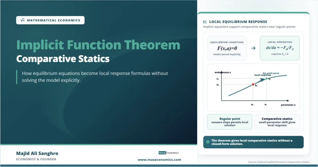
The theorem is one of the main mathematical tools behind equilibrium analysis. It shows when an equation such as \(F(x,a)=0\) can be treated locally as a function \(x=x(a)\), even if the model does not provide a closed-form solution for \(x\).
This matters because many economic models are solved implicitly. Supply and demand, consumer choice, firm optimization, macroeconomic equilibrium, and policy rules often define outcomes through conditions rather than explicit formulas. The implicit function theorem turns those conditions into local response formulas.
Equilibrium equations are often implicit
Economic models often begin with an equilibrium condition rather than an explicit solution. A market clears when demand equals supply. A firm chooses output where marginal revenue equals marginal cost. A household chooses a bundle where marginal rates and prices align. These conditions define outcomes, but they do not always solve directly for the variable of interest.
A simple market-clearing condition can be written as:
Market equilibrium condition
If the demand and supply functions are simple, the equation may be solved directly for \(P\). In many models, however, the equation is nonlinear, contains several variables, or belongs to a larger system. The solution exists as an equilibrium relationship, but not as a simple formula.
The implicit function theorem provides the local bridge. It asks whether the equilibrium condition \(F(P,Y)=0\) can be read near a point as \(P=P(Y)\). If so, the model can describe how equilibrium price changes when income changes, even without a closed-form expression for price.
Differentiation gives local movement
The theorem builds on differentiation. First derivatives measure how a function changes when one variable changes slightly. In an implicit equilibrium equation, the derivative must respect the condition that the equation remains true.
Suppose the equilibrium condition is:
Here, \(x\) is the endogenous variable and \(a\) is an exogenous parameter. If \(x\) changes when \(a\) changes, the total differential is:
Total differential
Solving for the response of \(x\) to \(a\) gives:
Implicit comparative-static derivative
This formula is the workhorse result. The parameter effect \(F_a\) shows how the equilibrium condition shifts directly. The slope term \(F_x\) shows how strongly the endogenous variable restores the equilibrium condition. The negative sign reflects the adjustment needed to keep \(F(x,a)=0\).
The theorem needs a nonzero slope
The one-equation version of the theorem requires three basic ideas. The function must be smooth enough near the point. The initial point must satisfy the equilibrium equation. The derivative with respect to the endogenous variable must not be zero.
One-equation condition
If these conditions hold, then near \((x_0,a_0)\), there exists a local function \(x=x(a)\) that keeps the equilibrium condition true:
The nonzero slope condition is essential. If \(F_x=0\), the equilibrium condition may be locally flat in the \(x\) direction. A small parameter change may produce no local solution, multiple local solutions, or an unstable jump. The usual comparative-static derivative may fail.
Economically, \(F_x\neq 0\) means the endogenous variable has enough local effect on the equilibrium condition to restore balance after a small shock. In a market model, price must actually affect excess demand. If price has no local effect, price cannot perform the local adjustment role.
A local diagram clarifies
The theorem is local. It does not claim that a single function exists everywhere. It says that near a regular equilibrium point, the equation can be treated as a function for small changes.

The diagram shows an implicit equilibrium curve. Each point on the curve satisfies \(F(x,a)=0\). When the parameter changes from \(a_0\) to \(a_1\), the theorem explains when the model can trace a nearby equilibrium change from \(x_0\) to \(x_1\).
Comparative statics follows directly
Comparative statics studies how equilibrium changes when an outside parameter changes. The implicit function theorem gives the derivative needed for that exercise.
In a market model, suppose equilibrium is written as excess demand equal to zero:
Excess demand equilibrium
The response of equilibrium price to income is:
Price response to income
If income raises demand, then \(F_Y>0\). If a higher price reduces excess demand, then \(F_P<0\). The derivative is positive:
The result matches economic intuition. Higher income shifts demand outward, and equilibrium price rises when price restores market balance. The theorem makes the logic formal without requiring an explicit price formula.
The denominator measures adjustment strength
The denominator in the comparative-static formula is not a technical detail. It measures how strongly the endogenous variable affects the equilibrium condition.
In the formula:
\(F_a\) is the direct shift from the parameter. \(F_x\) is the local adjustment force. If \(|F_x|\) is large, the endogenous variable strongly affects the equilibrium condition, so only a small change in \(x\) is needed to offset the shock. If \(|F_x|\) is small, the same shock can require a large change in \(x\).
This is why flat equilibrium conditions can create large comparative-static effects. A small policy or demand shock may produce a large change in price, quantity, or output when the restoring slope is weak.
If \(F_x=0\), the usual formula breaks down. The theorem no longer guarantees a smooth local function. Economic interpretation then requires a different method, such as higher-order analysis, a graphical inspection, or a broader equilibrium selection argument.
Several variables require matrices
Many economic models contain several endogenous variables. In that case, the implicit function theorem uses the Jacobian matrix. Suppose the model is:
System of equilibrium equations
The total differential is:
If the Jacobian \(F_x\) is nonsingular, then the local response is:
System comparative statics
This is the system version of the one-equation result. The scalar denominator \(F_x\) becomes a Jacobian matrix. The condition \(F_x\neq 0\) becomes \(\det(F_x)\neq 0\).
The economic meaning is the same. The model must contain enough independent local equations to pin down the endogenous variables. If the Jacobian is singular, the ordinary local comparative-static calculation cannot be used directly.
Optimization uses the same theorem
The implicit function theorem also supports optimization techniques. First-order conditions often define optimal choices implicitly as functions of prices, income, wages, interest rates, or policy parameters.
For example, a firm’s optimal input demand may be defined by:
Input demand condition
This condition may define labor demand \(L=L(w)\). The implicit derivative is:
Since \(F_w=-1\), the sign depends on \(F_L\). If marginal product is diminishing, then \(F_L=P\cdot MP_{LL}<0\), so:
The result says that a higher wage reduces labor demand under the standard diminishing-marginal-product condition. The theorem converts the first-order condition into a local demand response.
Demand functions are implicit solutions
Consumer theory provides another important example. A household maximizes utility subject to a budget constraint. The first-order conditions and the budget equation jointly determine demands for goods.
For a two-good interior solution, the system may be written as:
Consumer first-order system
The solution gives Marshallian demands \(x=x(p_x,p_y,m)\) and \(y=y(p_x,p_y,m)\), but those demand functions may not always have simple closed forms. The implicit function theorem gives conditions under which the local demand functions exist and can be differentiated.
This is the mathematical reason comparative statics in consumer theory can proceed from first-order conditions. A price or income change affects the equations directly, and the endogenous quantities adjust to restore both tangency and budget feasibility.
The theorem therefore sits quietly behind many standard economic results. Demand slopes, income effects, input demand responses, and policy multipliers often rely on implicit differentiation rather than explicit solutions.
The theorem is local only
The implicit function theorem is a local result. It says that a function exists near a particular regular point. It does not guarantee that the same function exists globally over the whole domain.
A model may have a clean local response near one equilibrium and fail elsewhere. Curves can fold, become vertical, cross multiple times, or generate several equilibria. The theorem does not eliminate those possibilities.
This distinction matters in economics because local comparative statics can be precise but limited. A small tax change near a stable equilibrium may have a well-defined effect. A large policy shock may move the economy into a different region where the original derivative no longer applies.
For this reason, comparative statics derived from the theorem should be interpreted as marginal responses around a specified equilibrium, not as universal predictions for all possible changes.
Nonzero conditions prevent breakdown
The theorem’s nonzero derivative or nonsingular Jacobian condition prevents several breakdowns. If the condition fails, the equilibrium relation may not be a function. One parameter value may correspond to several nearby endogenous values. The curve may turn vertical. The system may lose rank.
A simple example is:
For \(a>0\), there are two branches, \(x=\sqrt{a}\) and \(x=-\sqrt{a}\). At \(a=0\), the derivative \(F_x=2x\) equals zero. The theorem does not apply at \((0,0)\). The equilibrium relation has a turning point, and local uniqueness fails.
Economic models can show the same issue. Multiple equilibria, tipping points, liquidity traps, binding constraints, and discontinuous adjustment can all weaken ordinary local comparative statics.
Caveat. The implicit function theorem does not rule out multiple equilibria or large nonlinear changes. It gives a local result around a regular point where the relevant derivative or Jacobian is nonzero.
Policy multipliers use the logic
Many policy multipliers are implicit-function results. A macroeconomic model may define equilibrium output through an equation involving output, interest rates, fiscal policy, and expectations. The multiplier measures how output changes when a policy parameter changes.
In a reduced-form equilibrium condition:
the government-spending multiplier is:
Policy multiplier
The numerator captures the direct effect of government spending on the equilibrium condition. The denominator captures the system’s feedback through output. A strong stabilizing feedback can reduce the multiplier. A weak feedback can enlarge it.
This structure appears across macroeconomics, public finance, labor economics, and international economics. The theorem is not tied to one field. It is a general tool for extracting local predictions from equilibrium conditions.
Comparative statics require interpretation
The theorem supplies a derivative, but economics supplies the interpretation. The signs and magnitudes of \(F_x\), \(F_a\), and the Jacobian entries depend on behavioral assumptions, market structure, and institutional details.
For example, the sign of a price response depends on demand and supply slopes. The sign of labor demand response depends on marginal productivity. The sign of a policy multiplier depends on spending behavior, tax responses, monetary policy, and expectations.
A correct derivative formula is therefore not enough. The model must justify the signs of the derivative terms. It must also identify the equilibrium point around which the derivative is being evaluated.
The implicit function theorem is best read as a disciplined method. It organizes local comparative statics, but it does not replace economic reasoning about why the underlying derivatives have particular signs.
The result guides model checking
The theorem also provides a useful diagnostic for model building. If a model’s equilibrium conditions cannot satisfy the nonzero derivative or nonsingular Jacobian requirement, standard comparative statics may not be valid.
This often reveals a missing equation, a redundant condition, or an unresolved normalization. In general equilibrium models, for example, one price may need to be normalized because only relative prices matter. In macroeconomic systems, a policy rule may be needed to close the model.
The theorem therefore helps identify whether the model is locally well-posed. A well-posed model does not guarantee empirical truth, but it gives a coherent mathematical basis for asking how equilibrium changes after a shock.
This is why implicit-function logic is common in advanced economic theory, numerical modeling, and applied structural work. It checks whether equilibrium conditions can support local solution and comparative-static analysis.
Explains
Three concepts behind implicit functions
Related mathematical economics concepts are developed across the MASEconomics library.
Explore the MASEconomics BlogConclusion
Implicit function theorem economics explains how economists derive local comparative statics from equilibrium conditions that are not solved explicitly. If the relevant derivative or Jacobian is nonzero, an implicit equation can be treated locally as a function, and its response to parameter changes can be calculated.
The theorem matters because many economic outcomes are defined by conditions rather than closed-form formulas. Market clearing, first-order conditions, policy rules, and dynamic steady states often determine variables implicitly. The theorem makes those relationships usable for local analysis.
Its limits are just as important as its power. The result is local, requires regularity, and does not remove multiple equilibria or nonlinear breakdowns. It provides the mathematical permission for comparative statics, while the economic model determines the meaning of the derivative.
Frequently Asked Questions
What is the implicit function theorem in economics?
The implicit function theorem shows when an equilibrium equation such as \(F(x,a)=0\) can be treated locally as a function \(x=x(a)\), allowing comparative statics without an explicit solution.
Why is the theorem useful for comparative statics?
It gives the derivative of an endogenous variable with respect to a parameter while keeping the equilibrium condition satisfied. This makes local equilibrium responses mathematically precise.
What is the basic implicit derivative formula?
For one equation \(F(x,a)=0\), the local derivative is \(dx/da=-F_a/F_x\), provided \(F_x\neq 0\) at the equilibrium point.
What happens if the derivative is zero?
If the relevant derivative is zero, the theorem may not apply. The equilibrium relation may fail to be locally unique, and ordinary comparative statics may be invalid.
How does the theorem work in systems?
In systems, the scalar derivative condition becomes a nonsingular Jacobian condition. If the endogenous-variable Jacobian is invertible, local comparative statics can be computed using the inverse Jacobian.
Did you find this article helpful? Share it with someone who loves economics. And remember, at MASEconomics, we make complex ideas simple.