On October 19, 1987, the Dow Jones Industrial Average fell 22.6 percent in a single trading session. Standard risk models, calibrated on the normal distribution, assigned that event a probability of roughly one in 10 to the 50th power, a number larger than the estimated count of atoms in the observable universe. The crash happened anyway. Two decades later, in 2008, mortgage-backed securities rated AAA by every major agency defaulted in waves that the underlying statistical models had deemed practically impossible.
Probability distributions economics sit at the centre of these stories. A distribution is the mathematical object that tells you which outcomes are likely, which are rare, and how rare the rare ones really are. Get the distribution wrong, and every downstream calculation, from a portfolio’s value-at-risk to a country’s poverty headcount, inherits the error. Get it right, and the same tool that priced a 1987 option helps a labour economist measure inequality, a central banker stress-test a bank, and an econometrician decide whether a coefficient is statistically distinguishable from zero.
This guide walks through the distributions that do most of the heavy lifting in modern economics, from the workhorse normal curve to the fat-tailed Pareto laws that govern wealth and financial returns. The goal is practical: knowing which distribution fits which problem, and recognising the moments when the textbook default will mislead you.
What a Probability Distribution Is
A probability distribution assigns probabilities to the possible values of a random variable. For a discrete variable, such as the number of patents a firm files in a year, the distribution is a list of probabilities summing to one. For a continuous variable, such as a stock return, the distribution is described by a probability density function (PDF), and probabilities are computed as areas under the curve.
Two summary objects do most of the work. The cumulative distribution function (CDF), \( F(x) = P(X \leq x) \), gives the probability that the variable falls at or below \( x \). The PDF, \( f(x) \), is the derivative of the CDF for continuous variables. Moments of the distribution, the mean \( E[X] \), the variance \( \text{Var}(X) \), the skewness, and the kurtosis, condense its shape into a few numbers.
Economics leans on distributions for four recurring reasons. Asset returns and consumption growth are random, so portfolio choice and optimal consumption require distributional assumptions. Cross-sectional variables like income, firm size, and city population are unevenly spread, and any inequality measure depends on which distribution is fitted. Regression errors are modelled as random draws, and the validity of standard errors, p-values, and confidence intervals in simple linear regression depends on the distribution of those errors. Risk and insurance pricing, examined in risk, uncertainty, and insurance, are quoted in expected losses, which only exist once a distribution is specified.
The choice between discrete and continuous matters. Counts of bankruptcies, default events, and labour-market transitions are discrete. Wages, GDP growth rates, and exchange-rate changes are usually treated as continuous, even though measurement is granular in practice. The distinction governs which estimator to use and which probability statements are legitimate.
The Workhorses of Applied Economics
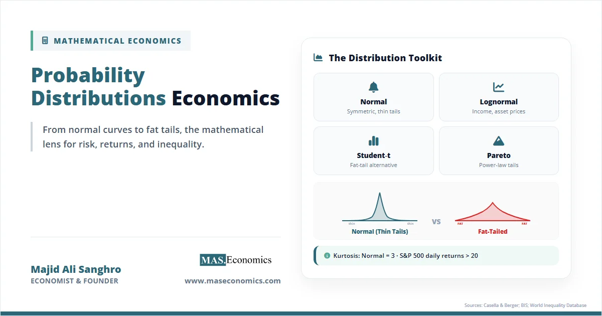
Three continuous distributions account for most empirical work in economics. The normal distribution is the default for errors and aggregated outcomes. The lognormal distribution handles positive-valued variables whose logarithm is approximately normal. The Student-t distribution provides fatter tails when sample sizes are small or when financial data refuse to behave.
The Normal Distribution
The normal distribution has the PDF
where \( \mu \) is the mean and \( \sigma^2 \) the variance. Its dominance in applied work comes from the central limit theorem (CLT): when many independent shocks combine additively, their sum tends toward a normal distribution regardless of the individual shocks’ shapes. The CLT is the reason ordinary least squares (OLS) coefficients in multiple regression models are approximately normal in large samples even when the underlying errors are not.
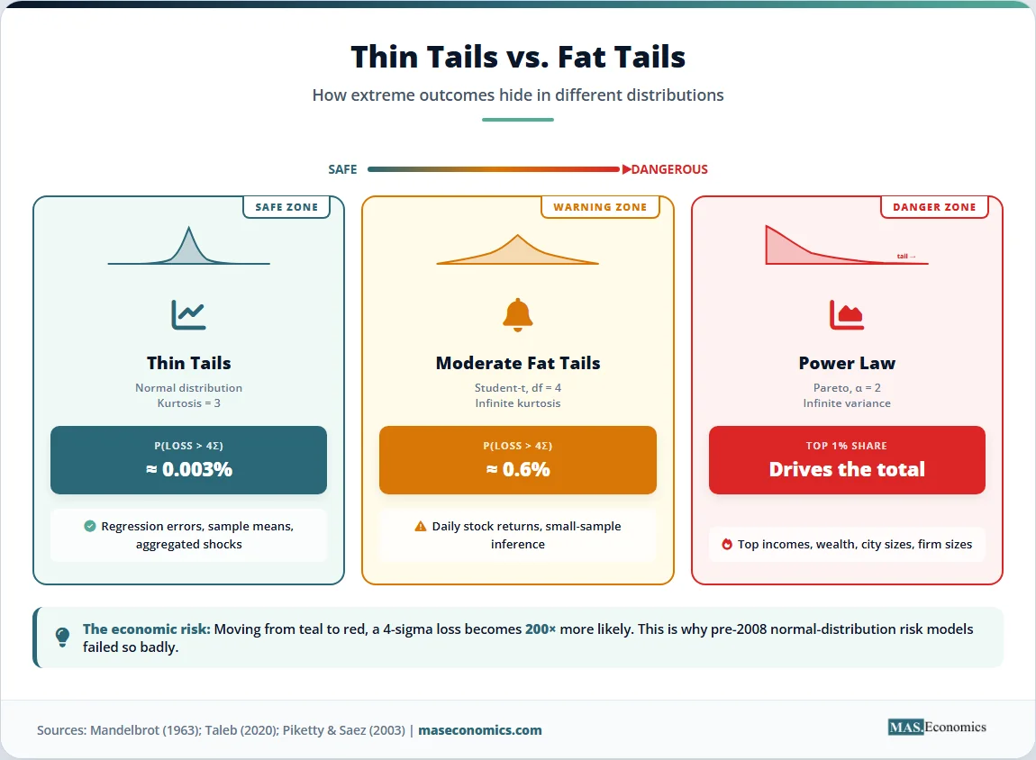
The normal has thin tails. Outcomes more than three standard deviations from the mean occur with probability about 0.0027. A six-sigma event has a probability below one in 500 million. These numbers are accurate when the data-generating process really is normal, and disastrously misleading when it is not.
The Lognormal Distribution
Many economic variables cannot be negative: income, wealth, asset prices, firm revenues, and durations of unemployment. A natural model is to assume that the logarithm of the variable is normally distributed, so the variable itself follows a lognormal distribution with PDF
The lognormal has a long right tail and a positive skew. It fits middle-of-the-distribution incomes reasonably well in many countries and underpins the geometric Brownian motion assumption used in the Black-Scholes option pricing model. Where it fails is at the very top: empirical income and wealth distributions have heavier upper tails than the lognormal predicts.
The Student-t Distribution
The Student-t distribution looks like a bell curve but with fatter tails. Its shape is governed by a single parameter, the degrees of freedom \( \nu \). As \( \nu \to \infty \), the t-distribution converges to the normal. For small \( \nu \), say four or five, tail probabilities are several times larger than the normal’s.
The t-distribution arises naturally in two settings. In small-sample inference, the standardised sample mean of normally distributed data follows a t-distribution rather than a normal one, which is why t-tables exist. In financial econometrics, daily returns are routinely modelled with a t-distribution because their empirical kurtosis is far above three, the value of the normal forces.
When Normality Fails
The normal distribution captures aggregate behaviour well when shocks are independent and bounded. Financial markets, income data, and firm-size distributions violate at least one of those conditions. The result is fat tails: extreme outcomes occur far more often than the normal predicts.
Kurtosis measures this. For a random variable with mean \( \mu \) and variance \( \sigma^2 \), the kurtosis is
The normal distribution has kurtosis exactly three. Daily returns on the S&P 500 have sample kurtosis well above 20 over long historical windows, and the figure rises sharply if crisis periods are included. A model that assumes normality, therefore understates the probability of large losses by orders of magnitude.
Power-law distributions provide the alternative. A variable \( X \) follows a power law if
where \( \alpha \) is the tail exponent. The Pareto distribution is the canonical example. When \( \alpha \leq 2 \), the variance is infinite. When \( \alpha \leq 1 \), even the mean does not exist in the usual sense. These are not pathological curiosities. Empirical estimates put the tail exponent of the U.S. wealth distribution near 1.5, of city populations near 1.0 (Zipf’s law), and of firm sizes near 1.1.
Three implications follow. First, sample averages converge slowly or not at all when \( \alpha \) is small. A single observation can dominate the sample mean. Second, the central limit theorem in its classical form does not apply, so OLS standard errors built on it are unreliable. Third, risk measures based on normal approximations, including the value-at-risk used by most banks before 2008, can underestimate true tail losses by factors of ten or more.
Benoit Mandelbrot first documented fat tails in cotton prices in the 1960s. Nassim Taleb’s Statistical Consequences of Fat Tails develops the practical implications, arguing that much of standard statistics simply does not work in the power-law regime. The work of Thomas Piketty and Emmanuel Saez on top-income shares, summarised at the World Inequality Database, shows that the top one percent’s share of income in many advanced economies is governed by a Pareto tail rather than a lognormal body, which is why small changes in tax policy at the top can produce large changes in measured inequality.
Discrete Distributions in Economics
Several discrete distributions appear repeatedly in applied work, each tied to a specific kind of economic question.
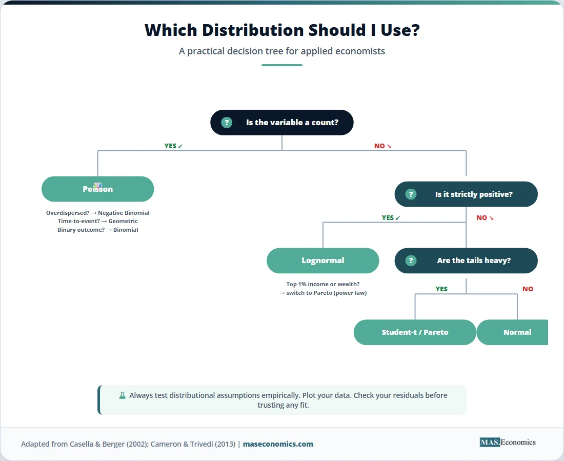
The binomial distribution counts successes in \( n \) independent trials with success probability \( p \). It underpins logit and probit models for binary outcomes: whether a household defaults on a loan, whether a worker participates in the labour force, and whether a country experiences a banking crisis in a given year. Maximum likelihood estimation of these models relies on the binomial probability mass function
The Poisson distribution models counts of rare events when the per-period probability is small, and events are independent. Patent counts by firm, sovereign defaults per year, and corporate bankruptcies per industry are common applications. Its PDF is
where \( \lambda \) is both the mean and the variance. That equality is restrictive: when observed counts are more dispersed than the Poisson allows, the negative binomial distribution is the standard fix.
The geometric distribution describes the number of trials until the first success. In labour economics, it models the duration of unemployment under the simplifying assumption that the exit probability per period is constant. Hazard models generalise it by allowing the exit probability to vary with elapsed time, capturing the empirical fact that long-term unemployed workers find jobs at lower rates than the recently unemployed.
These three distributions share a structural feature: they assume independence between events. When defaults cluster, when bankruptcies arrive in waves, or when patent filings spike around a regulatory change, the independence assumption breaks, and richer models are needed.
Comparing Tail Behaviour Visually
The contrast between thin and fat tails is easier to see than to describe. The chart below plots a standard normal density against a Student-t density with four degrees of freedom and a Pareto tail. The bodies of the three curves are similar. The tails tell a different story.
Source: Author’s calculations. Standard normal, Student-t with 4 df, and Pareto (alpha = 2, plotted from x = 1.5) shown on the same vertical scale to compare tail thickness.
At \( x = 4 \), the normal density is essentially zero. The Student-t still assigns meaningful probability to that region, and the Pareto tail decays so slowly that values far beyond four standard deviations remain plausible. For risk management, the gap between the red curve and the teal curve is the gap between underestimating crisis losses and pricing them realistically.
Distribution Cheat Sheet for Economists
The table below summarises the distributions most commonly used in applied economics, their key properties, and the contexts where each is appropriate.
| Distribution | Type | Key Parameters | Economic Application | Watch Out For |
|---|---|---|---|---|
| Normal | Continuous | Mean, variance | Regression errors, aggregated shocks, hypothesis tests | Underestimates tail risk in finance |
| Lognormal | Continuous, positive | Log-mean, log-variance | Wages, asset prices, firm revenues | Misses very top of income distribution |
| Student-t | Continuous | Degrees of freedom | Small-sample inference, financial returns | Variance undefined for df below 3 |
| Pareto | Continuous | Scale, tail exponent | Top incomes, wealth, city sizes, firm sizes | Mean infinite when alpha below 1 |
| Binomial | Discrete | Trials, success probability | Default events, binary choices, probit/logit | Independence assumption often violated |
| Poisson | Discrete | Rate parameter | Patent counts, defaults per year, accidents | Forces mean = variance |
| Geometric | Discrete | Success probability | Unemployment durations, time-to-event models | Constant hazard rare in real data |

|
||||
The Econometrics Connection
Distributions enter econometrics at three levels: the data, the estimator, and the test statistic. Each layer rests on a distributional assumption, and shifting one assumption ripples through the others.
Maximum likelihood estimation (MLE) requires a fully specified distribution for the data. Given parameters \( \theta \) and observations \( x_1, \ldots, x_n \), the log-likelihood is
The MLE \( \hat{\theta} \) maximises \( \ell(\theta) \). Under regularity conditions, \( \hat{\theta} \) is asymptotically normal with variance equal to the inverse Fisher information. That asymptotic normality is what justifies standard errors, t-statistics, and likelihood-ratio tests in logit, probit, and other binary-choice models.
Hypothesis testing uses three sampling distributions in particular. The t-distribution governs tests of single coefficients in small samples. The F-distribution governs joint tests of multiple coefficients, including the standard test for whether a regression has any explanatory power. The chi-squared distribution governs likelihood-ratio and Wald tests for nonlinear restrictions, and is the asymptotic distribution of the score test. All three are derived from the normal distribution under specific transformations: the t is a normal divided by a scaled chi-squared, the F is a ratio of two scaled chi-squared variables, and the chi-squared is a sum of squared normals.
Confidence intervals inherit the same architecture. A 95 percent interval for a parameter is, in most cases, the point estimate plus or minus 1.96 standard errors, where 1.96 is the 97.5th percentile of the standard normal. If the true sampling distribution has fatter tails, that interval undercovers: the nominal 95 percent confidence level becomes a lower true coverage rate. This is one reason robust standard errors and bootstrap methods have spread through applied work.
Distributional misspecification is rarely benign. Assuming normality when errors are fat-tailed inflates apparent precision and produces overconfident inferences. Assuming a Poisson distribution when counts are overdispersed produces standard errors that are too small, which means significant findings that are not really significant. The discipline of asking “what distribution does my model assume, and does the data plausibly come from it?” is among the most useful habits an applied economist can develop.
Where Distribution Choice Bites Hardest
Three areas illustrate why distributional choices have real consequences. The first is financial risk management. Bank value-at-risk models built on the normal distribution before 2008 assigned tiny probabilities to the simultaneous default of mortgage pools that turned out to be highly correlated. A 1995 Basel Committee framework permitted internal models with normal-distribution assumptions, and the resulting capital requirements proved inadequate when correlations spiked. Post-crisis revisions, including the 2019 Fundamental Review of the Trading Book, replace value-at-risk with expected shortfall and require stressed calibration, partly to address the failure of thin-tailed assumptions.
The second is inequality measurement. Gini coefficients computed under a lognormal assumption diverge sharply from those computed under a Pareto-tailed model, because the top one percent’s share is pinned down by the tail exponent. Piketty, Saez, and their collaborators have shown that the share of national income captured by the top one percent in the United States rose from roughly 10 percent in 1980 to above 20 percent by the mid-2010s, a movement that the standard lognormal cannot generate. Policy debates over wealth taxation depend on which distribution is fitted to the upper tail.
The third is event-count modelling in industrial organisation and labour economics. A Poisson model of patent counts assumes that any firm’s filings are independent across time, with a stable rate. In reality, firms cluster their filings around acquisitions, regulatory deadlines, and product launches. Negative binomial and zero-inflated models, which relax the Poisson’s mean-equals-variance constraint, frequently change the sign or significance of the policy variables of interest. The same point applies to default counts in credit risk and accident counts in insurance.
Limits of the Standard Toolkit
Knowing many distributions is necessary but not sufficient. Three limits are worth keeping in view.
Independence assumptions are routinely violated. The normal, the Poisson, and the binomial all assume that draws are independent. Financial returns exhibit volatility clustering. Defaults arrive in waves. Patent filings respond to common shocks. Models that ignore dependence understate uncertainty even when the marginal distribution is correctly specified.
Stationarity is fragile. Many econometric techniques assume that the distribution generating the data does not change over time. Regimes shift. The distribution of inflation in the 1970s differs from that in the 1990s. Structural breaks in time series analysis are explicit attempts to model these shifts, but they cannot do so when the break is unprecedented.
Estimation of tail behaviour is hard precisely because tail data are rare. The Hill estimator and other tail-index methods produce wide confidence intervals when only a handful of observations lie in the tail. Stating that a series follows a power law with \( \alpha = 2.3 \) is honest only if the standard error around 2.3 is reported, which it often is not.
MASEconomics Explains
Four economic concepts behind probability distributions
Conclusion
Probability distributions economics is the language in which uncertainty, risk, and inequality are quantified. The normal distribution remains the natural default for many estimators because the central limit theorem keeps doing its work. The lognormal handles positive variables across most of their range. The Student-t accommodates heavy-tailed data with a single tunable parameter. Power laws describe the upper tails of income, wealth, and firm-size distributions, and they imply behaviour that thin-tailed models cannot capture.
The 2008 crisis and the long history of financial panics show what happens when distributional assumptions are wrong. The growth of inequality research in the last two decades shows what becomes visible when the right distribution is fitted. The choice between distributions is not a technical footnote. It determines what counts as a rare event, how confident an estimate really is, and whether a policy debate is grounded in the data or in a convenient fiction.
Did you find this article helpful? Share it with someone who loves economics. And remember, at MASEconomics, we make complex ideas simple.