Spurious Regression: When Trends Create False Relationships

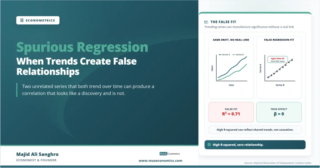
In 1926, the statistician George Udny Yule presented a puzzle to the Royal Statistical Society. Between 1866 and 1911, the share of marriages in England performed by the Church of England fell steadily, and over the same decades the national mortality rate fell steadily too. Run a correlation between the two and you get 0.95, a figure so high that any conventional test would call it overwhelmingly significant. Yet no one believes that civil weddings kept people alive, or that church weddings killed them. The two series had nothing to do with each other. They simply drifted downward together across the same half-century, and that shared drift was enough to manufacture a correlation that looked like a discovery. This is the classic illustration of spurious regression: a statistically significant relationship between variables that are not actually related, produced by the way each variable moves over time rather than by any genuine connection between them.

The problem is not a curiosity from the early history of statistics. It is one of the most common ways that time-series analysis goes wrong, and it is dangerous precisely because the symptoms mimic success. A spurious regression typically produces a large t-statistic, a high R-squared, and a coefficient that looks economically meaningful. Everything the analyst was trained to look for as evidence of a real effect is present, and all of it is an illusion. Understanding why this happens, and how to detect it, is one of the foundations of working with economic time series.

Why Trending Series Correlate by Accident

The root of the problem is that many economic time series are nonstationary. A stationary series fluctuates around a constant mean with a stable variance, so that its statistical behavior today looks like its behavior a decade ago. A nonstationary series does not. The most important case is the random walk, where each value equals the previous value plus a random shock, so that shocks accumulate permanently rather than dying out.

Random Walk With Drift

Each shock \(\varepsilon_t\) is added to the running total and never fades. The drift term \(\alpha\) gives the series a persistent tendency to move in one direction, producing a visible trend.

Consider two independent random walks generated by completely separate streams of random shocks. By construction, they have no relationship whatsoever. But each one wanders away from its starting point and tends to keep moving in whatever direction its accumulated shocks have pushed it. Over any given sample, one will probably drift upward while the other drifts upward too, or both downward, or one up and one down. Whatever the pattern, a straight line fitted between them will usually find apparent structure, because two series that both trend will line up against each other far more often than chance would suggest for two stationary series.

The reason this fools the standard regression machinery is subtle. Ordinary least squares assumes the regression errors are well behaved, in particular that they do not themselves carry a trend. When both the dependent and independent variables are nonstationary and unrelated, the regression residuals inherit the nonstationarity. The errors are not random noise around the fitted line; they are themselves a wandering, trending series. This violates the assumptions that make the usual t-statistics and standard errors valid, and the violation is not mild. The whole inferential apparatus breaks.

The Statistics That Should Warn You, and Why They Do Not

The deepest result in this area is that the diagnostic tools an analyst would normally trust point in exactly the wrong direction under spurious regression. Granger and Newbold demonstrated this with simulations in their 1974 paper, and Peter Phillips later proved the asymptotic theory behind it. The finding is that the conventional t-statistic and F-statistic from a regression of one independent random walk on another do not settle down to stable distributions as the sample grows. They diverge. The larger the sample, the larger the t-statistic tends to become, which means that collecting more data makes a false relationship look more convincing rather than less.

This inverts the intuition that more data is always safer. With stationary series, a larger sample sharpens estimates and exposes relationships that are not real as statistically insignificant. With nonstationary series in a spurious regression, a larger sample inflates the apparent significance of a relationship that does not exist. The t-statistic that would normally reassure the analyst is, in this setting, the very thing producing the false confidence.

Table 1. Genuine Relationship Versus Spurious Regression

Diagnostic	Genuine relationship (stationary)	Spurious regression (two random walks)
R-squared	Reflects true explanatory power	Often high, but meaningless
t-statistic	Stabilizes; falls toward zero if no effect	Diverges; grows with sample size
Durbin-Watson statistic	Near 2 when errors are clean	Near 0, signalling trending residuals
Residuals	Stationary noise around the line	Nonstationary; wander and trend
Reliable conclusion	Standard inference valid	Standard inference invalid
Source: Properties summarised from Granger and Newbold (1974) and Phillips (1986).

The Durbin-Watson statistic deserves a special mention, because it is the one diagnostic that does sound the alarm. A Durbin-Watson value far below 2, particularly close to 0, indicates strongly autocorrelated residuals, which is the fingerprint of trending errors. Granger and Newbold proposed a memorable rule of thumb: if the R-squared exceeds the Durbin-Watson statistic, the regression should be treated with deep suspicion. A high R-squared paired with a very low Durbin-Watson is the combination that should make an analyst stop rather than celebrate.

A Worked Example: Two Series That Share Nothing

Consider a stylized example with internally consistent numbers. Two series are generated as independent random walks, each from its own separate set of random shocks, so that the true relationship between them is exactly zero. An analyst who did not know how the data were generated regresses the first on the second and reads off the output.

Table 2. Regressing One Independent Random Walk on Another

Output statistic	Value	How it looks	What is actually true
Slope coefficient \(\hat{\beta}\)	0.82***	Large and highly significant	True value is zero
Standard error	(0.06)	Tight, suggesting precision	Invalid; based on broken assumptions
t-statistic	13.7	Far beyond any critical value	Diverges with sample size
R-squared	0.71	Strong fit	Explains nothing real
Durbin-Watson	0.18	The one red flag	Confirms trending residuals
Verdict	—	Looks like a strong result	Entirely spurious
Source: Stylized example based on standard formulas. Numbers chosen for illustration.

Every headline number in this output is the kind that an empirical economist would normally treat as a finding worth reporting. The coefficient is large, the t-statistic is enormous, and the R-squared is high. Only the Durbin-Watson statistic, sitting at 0.18 against an ideal of around 2, betrays the truth. The residuals are not clean noise; they are a wandering series that trends along with the regressors. The relationship is an artifact of two series drifting through the same window of time, and nothing more.

Unit Roots: The Source of the Trouble

The formal language for this problem is the unit root. A series has a unit root when the coefficient on its own lagged value equals one, which is exactly the random-walk case where shocks accumulate without decay. A series with a unit root is integrated of order one, written \(I(1)\), meaning it must be differenced once to become stationary. Spurious regression arises specifically when two \(I(1)\) series that are not genuinely linked are regressed on each other in levels.

This is why the diagnosis runs through testing for unit roots before running a levels regression. The question to ask of any economic time series is whether it is stationary or whether it contains a unit root, and the answer determines whether ordinary regression in levels is even permissible. The properties that make a series safe or dangerous for regression are exactly the properties covered in the treatment of stationarity in time-series econometrics. A series that is stationary can be regressed on another stationary series with the usual tools. A pair of unit-root series cannot, unless a further condition holds.

Detecting and Avoiding the Trap

The practical workflow has a clear order. The first step is to test each series for a unit root before running any regression in levels. The standard tool is the Augmented Dickey-Fuller test, which tests the null hypothesis that a series contains a unit root against the alternative that it is stationary. If the test fails to reject the null for both series, the analyst is in dangerous territory and must not interpret a levels regression at face value.

The most common fix is to difference the series. Taking first differences of an \(I(1)\) series, that is, working with the change from one period to the next rather than the level, usually produces a stationary series on which ordinary regression is valid. Differencing removes the accumulated trend that drives the spurious correlation. The cost is that differencing discards information about the long-run levels of the variables, and it answers a different question: it describes how changes relate to changes, not how levels relate to levels.

There is one important exception that rescues levels regressions in special cases. Two \(I(1)\) series can be genuinely linked if they share a common stochastic trend, so that a particular linear combination of them is stationary even though each series individually is not. This is cointegration, and it is the line that separates a spurious regression from a meaningful long-run relationship. When two series are cointegrated, regressing one on the other in levels is not spurious; it estimates a real equilibrium relationship. The methods for testing this directly, and for modeling the short-run dynamics around the long-run equilibrium, are developed in the treatment of cointegration and the Engle-Granger method. The whole apparatus of cointegration exists precisely to tell apart two cases that look identical in a raw levels regression: a false relationship between drifting series and a true one between series tied together over the long run.

Where Spurious Regression Sits in the Toolkit

Spurious regression is one of the clearest illustrations of why the assumptions behind a method matter as much as the method itself. The mechanics of fitting a line are the same whether the underlying series are stationary or not, which is exactly why the trap is so easy to fall into. The foundations of fitting and interpreting that line are covered in the treatments of simple linear regression and multiple regression models, and the spurious-regression problem is best understood as what happens when the data fed into those models violate the conditions those models assume.

The problem also connects to the wider question of what a statistical relationship between time series actually means. A high correlation between two trending variables tells us nothing about whether one helps predict the other once their trends are accounted for, which is the question that Granger causality was designed to address, and which itself requires stationary inputs to be meaningful. Seen in this company, spurious regression is not an isolated pitfall. It is the canonical reminder that economic time series carry structure across time, and that ignoring that structure turns the ordinary tools of regression into machines for generating confident nonsense.

Explains

Conclusion

The danger of spurious regression is that it counterfeits every sign of a genuine result. A regression of one nonstationary series on another unrelated nonstationary series typically delivers a large coefficient, a small standard error, a t-statistic that grows with the sample, and a high R-squared. The trended residuals that should expose the problem are invisible unless the analyst inspects them, and the single diagnostic that does flag the trouble, a Durbin-Watson statistic near zero, is easy to overlook in the glow of an apparently strong fit. Yule’s nineteenth-century marriage and mortality series, correlated at 0.95 with no causal link whatever, remains the cleanest demonstration that shared movement over time is not evidence of a shared cause.

The defense is procedural and well established. Test each series for a unit root before interpreting any regression in levels, treat a high R-squared paired with a low Durbin-Watson as a warning rather than a triumph, and difference the series when they are nonstationary and not cointegrated. The one case in which a levels regression survives is cointegration, where a stationary linear combination ties the series together in a genuine long-run relationship. The lesson that runs through all of this is that the validity of a regression depends on the time-series properties of its inputs, and that with economic data those properties cannot be assumed. They have to be tested.

Frequently Asked Questions

Thanks for reading! If you found this helpful, share it with friends and spread the knowledge. Happy learning with MASEconomics