Why does a Big Mac cost $5.20 in Switzerland but only $1.05 in China when converted to dollars? Why does the Japanese yen appear so much stronger against the dollar today than it did in the 1970s? And why, despite these massive disparities, do exchange rates eventually seem to find their way back toward some underlying level?
For more than a century, economists have turned to a simple yet powerful idea to answer such questions: purchasing power parity (PPP). The concept is disarmingly intuitive; once converted to a common currency, national price levels should be equal. If a basket of goods costs more in one country than another, arbitrageurs will buy where it is cheap and sell where it is dear, forcing prices and exchange rates to align.
Yet the real world stubbornly defies this tidy logic. Currencies fluctuate wildly, price gaps persist for years, and the relationship between exchange rates and prices remains one of the most hotly debated topics in international economics. The purchasing power parity theory, born in the chaos of World War I, has been celebrated, dismissed, resurrected, and refined. Today it stands as a fundamental benchmark, a long‑run anchor that, despite its shortcomings, no serious analysis of exchange rates can ignore.
What Did Economists Believe?
Before World War I, the world operated under the gold standard. Most major currencies were convertible into gold at fixed parities, so the exchange rate between any two currencies was simply the ratio of their gold contents. If a British pound contained 4.866 grams of gold and a US dollar contained 1.505 grams, the exchange rate was fixed at $4.866 per pound. There was no question about what the “right” exchange rate should be; it was set by the mint.
When the war broke out, the gold standard collapsed. Governments printed money to finance the war effort, and inflation soared. By 1918, the German mark had lost half its value, the French franc a third, and the British pound had also depreciated. Countries faced an unprecedented problem: how to restore order to their exchange rates? Returning to prewar parities made no sense because the relative purchasing power of currencies had changed dramatically.
Into this vacuum stepped a Swedish economist named Gustav Cassel. He proposed a radical idea: exchange rates should be set so that the purchasing power of each currency, measured by its ability to buy a representative basket of goods, is the same. The ratio of price levels would determine the equilibrium exchange rate. This was the birth of purchasing power parity as a practical policy tool.
The Man Behind the Idea
Gustav Cassel (1866–1945) was a towering figure in Swedish economics. A professor at Stockholm University, he was one of the early proponents of the quantity theory of money and a fierce critic of the gold standard. During World War I, as inflation raged and exchange rates became disconnected from their gold parities, Cassel began developing a theory of exchange rate determination based on price levels.
In a 1916 article and later in his 1918 paper “Abnormal Deviations in International Exchanges,” Cassel introduced the term purchasing power parity. He argued that “the rate of exchange between two countries is primarily determined by the quotient between the internal purchasing power against goods of the money of each country.” In his 1922 book Money and Foreign Exchange After 1914, he expanded the theory and proposed using PPP calculations to guide the restoration of the international monetary system.
Cassel’s idea was simple yet powerful. If a currency’s purchasing power had halved because of inflation, its exchange rate should also halve. This gave policymakers a clear anchor: the equilibrium exchange rate was the one that equalized price levels. Although his specific prescriptions were not always followed, the concept of PPP became an essential part of the economist’s toolkit.
Absolute and Relative PPP
Purchasing power parity comes in two main versions: absolute and relative.
Absolute PPP
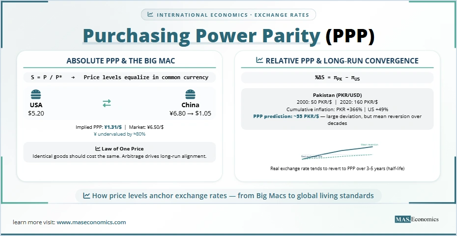
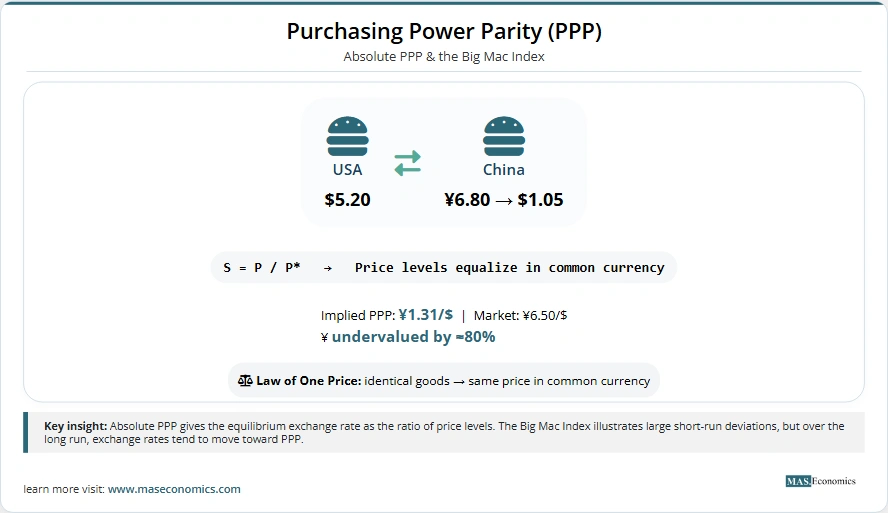
Absolute PPP states that the exchange rate between two currencies should equal the ratio of the price levels in the two countries. In symbols:
S = \frac{P}{P^*}
$$
where \(S\) is the nominal exchange rate (units of domestic currency per unit of foreign currency), \(P\) is the domestic price level, and \(P^*\) is the foreign price level. If a basket of goods costs $100 in the US and €80 in Germany, absolute PPP says the exchange rate should be $1.25 per euro.
This version implies that the real exchange rate, the nominal exchange rate adjusted for price differences, is always equal to one. The real exchange rate is defined as:
Q = \frac{S \cdot P^*}{P}
$$
If absolute PPP holds, \(Q = 1\).
Relative PPP
Relative PPP is a weaker condition. It says that the percentage change in the exchange rate should equal the difference between domestic and foreign inflation rates:
In words, if inflation is higher at home than abroad, the domestic currency should depreciate by approximately that difference. Relative PPP does not require that price levels be equal at any point in time; it only requires that they move together over time.
Relative PPP is more practical for empirical testing because it does not require a baseline year in which absolute PPP holds. Most modern research on PPP focuses on the behaviour of the real exchange rate: if PPP holds in the long run, the real exchange rate should be mean‑reverting.
The Law of One Price
The microeconomic foundation of PPP is the law of one price (LOP): identical goods should sell for the same price when expressed in a common currency. For a single good \(i\):
P_i = S \cdot P_i^*
$$
If LOP holds for all goods, and the same weights are used in the price indexes, then absolute PPP follows. But as we shall see, LOP fails spectacularly for many goods.
A MASEconomics Example
Consider the Pakistani rupee (PKR) and the US dollar. In 2000, the exchange rate was about 50 PKR per dollar. Suppose a typical Pakistani consumer basket costs 5,000 rupees, while a comparable US basket costs $100. Absolute PPP would imply an exchange rate of 50 PKR/$, which was roughly true at that time.
Fast‑forward to 2020. Inflation in Pakistan averaged about 8% per year, while US inflation averaged about 2%. Over 20 years, the cumulative price increase in Pakistan was about \((1.08)^{20} \approx 4.66\), or 366%, while in the US it was \((1.02)^{20} \approx 1.49\), or 49%. According to relative PPP, the rupee should have depreciated by approximately the inflation differential: \((1.366)/(1.49) \approx 0.917\), meaning the rupee should have weakened to about \(50 / 0.917 \approx 54.5\) rupees per dollar.
What actually happened? By 2020, the exchange rate was around 160 rupees per dollar, far more than the PPP prediction. This huge discrepancy reflects a combination of factors: productivity differences (the Balassa‑Samuelson effect), capital flows, political instability, and the fact that not all goods are traded.
This example illustrates the central puzzle of PPP: in the short run, exchange rates can deviate dramatically from the levels suggested by price differences, yet over very long horizons, they tend to converge.
The Balassa‑Samuelson Effect and Beyond
One of the most important refinements to PPP came from Bela Balassa (1964) and Paul Samuelson (1964). They argued that a simple comparison of aggregate price levels across countries is misleading because nontraded goods are cheaper in poor countries.
The Balassa‑Samuelson Hypothesis
Suppose a country experiences faster productivity growth in its traded goods sector (e.g., manufacturing) than in its nontraded sector (e.g., services). Wages in the traded sector rise to reflect higher productivity. Because labor is mobile across sectors, wages in the nontraded sector also rise, even though productivity there has not increased. As a result, the prices of nontraded goods rise relative to traded goods.
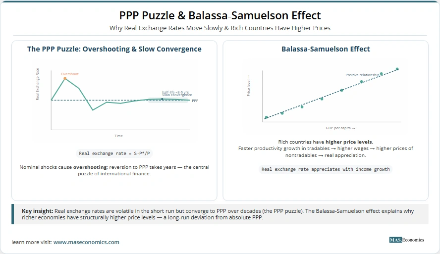
Now compare two countries. The richer country, with higher productivity in tradables, will have higher relative prices of nontradables. Its overall price level will therefore be higher when converted at the exchange rate. Consequently, absolute PPP will not hold; the rich country’s currency will appear overvalued when measured by a simple price comparison.
This is exactly what the data show: when you plot price levels against income per capita, there is a clear positive relationship. Rich countries have higher price levels. This “Penn effect” is now a stylised fact in international economics.
The Balassa‑Samuelson effect implies that the real exchange rate should appreciate as a country grows richer. For fast‑growing economies like Japan in the 1970s and 1980s, the real appreciation of the yen was partly driven by this productivity effect.
Nonlinear Adjustment and Transaction Costs
Another important extension is the recognition that adjustment to PPP may be nonlinear. If transaction costs, shipping, tariffs, and information costs create a band around the equilibrium, then small deviations will not be arbitraged away because the cost of doing so exceeds the profit. Only when the deviation becomes large enough to cover transaction costs will trade occur and prices converge.
This “band of inaction” leads to a process where the real exchange rate exhibits threshold autoregressive or smooth transition behaviour. Econometric models that allow for such nonlinearity find that the half‑life of deviations from PPP is much shorter, often less than two years for large shocks, which helps resolve the so‑called “PPP puzzle.”
Border Effects and Currency Unions
Research by Charles Engel and others has shown that even after controlling for distance, international price dispersion is much larger than domestic dispersion. The “border effect” is substantial: crossing a national border adds a large implicit barrier to price equalisation. However, when countries share a common currency, as in the eurozone, price dispersion is significantly reduced. This suggests that nominal exchange rate volatility is a major source of deviations from PPP.
The Challenge
Despite its intuitive appeal, PPP faces a series of empirical puzzles that have troubled economists for decades.
Short‑Run Volatility
In the short run, real exchange rates are extremely volatile. As shown in many studies, the US dollar/Deutsche Mark real exchange rate fluctuated wildly after 1973, with deviations often exceeding 30%. This volatility is driven largely by nominal exchange rate movements because nominal prices are sticky. In the famous Dornbusch overshooting model, a monetary shock causes the exchange rate to jump more than the underlying price levels, creating large temporary deviations from PPP.
The Glacial Speed of Convergence
The real puzzle is not the existence of short‑run deviations but their persistence. Estimates of the half‑life of PPP deviations, the time it takes for a shock to dissipate by 50%, have converged to a surprisingly narrow range of 3 to 5 years. This is far longer than the one to two years that many macroeconomists would expect, given sticky prices.
Why should it take so long for arbitrage to eliminate price differences? Possible explanations include:
- Transportation costs and tariffs: these create a wide band within which no arbitrage occurs.
- Pricing to market: firms may deliberately set different prices in different markets to maximise profits, adjusting prices slowly in response to exchange rate changes.
- Nontraded components: even “tradable” goods contain a large share of nontraded services (distribution, retailing), which are not subject to international arbitrage.
- Hysteresis: once firms exit a foreign market due to unfavourable exchange rates, they may not re‑enter quickly even when rates return to equilibrium.
Kenneth Rogoff’s 1996 Journal of Economic Literature survey crystallised the PPP puzzle: how can we reconcile the high short‑term volatility of real exchange rates with the extremely slow rate at which shocks seem to die out? The puzzle remains a central challenge in international finance.
Evidence from Long‑Horizon Data
Despite the short‑run failures, a vast body of research using long‑horizon data (often spanning a century or more) finds strong evidence of mean reversion. Studies by Frankel (1986), Lothian and Taylor (1996), and others have shown that real exchange rates do revert toward PPP over periods of several decades. The consensus is that PPP holds in the very long run, but the speed of convergence is indeed measured in years, not months.
PPP Today
The International Comparison Program and the Penn World Table
One of the most important practical applications of PPP is the construction of international price comparisons. The International Comparison Program (ICP), coordinated by the World Bank, collects detailed price data across countries to compute PPP exchange rates. These are used to convert GDP into a common currency for comparing living standards.
The Penn World Table, developed by Robert Summers and Alan Heston, has made these data widely available. It shows, for example, that when measured at PPP, the gap between rich and poor countries is much smaller than when measured at market exchange rates. This is because nontraded goods are cheaper in poor countries, so their GDP understates real consumption if converted at market rates.
The Big Mac Index
In 1986, The Economist introduced the Big Mac Index as a light‑hearted guide to whether currencies are over‑ or undervalued. The index compares the price of a McDonald’s Big Mac hamburger across countries. Because the Big Mac is produced to a standard recipe around the world, it provides a simple test of PPP.
The Big Mac Index often reveals large deviations. For example, in 2015, a Big Mac cost $5.20 in Switzerland but only $1.05 in China, implying the Swiss franc was overvalued and the yuan undervalued. Over time, these deviations tend to shrink, though slowly. The index has become a popular teaching tool and is even used by some currency traders as a rough guide.
PPP in Forecasting and Policy
Central banks and international institutions use PPP as a long‑run benchmark for exchange rate forecasts. Many models incorporate PPP as an equilibrium condition that binds in the long run. In practice, however, short‑term forecasting remains notoriously difficult; the random walk often outperforms structural models.
PPP also plays a role in debates over exchange rate regimes. Countries that peg their exchange rate may find that sustained inflation differentials lead to real overvaluation, eventually forcing a crisis. The Mexican peso crisis of 1994 and the Asian financial crisis of 1997–98 were preceded by large real appreciations, which PPP analysis could have flagged as warning signs.
Digital Trade and New Challenges
The rise of digital goods and services poses new questions for PPP. When a software subscription or a cloud service is sold globally, the law of one price should theoretically hold. Yet digital markets often exhibit price discrimination across countries due to different willingness to pay, taxes, and regulatory barriers. Whether PPP will hold for digital goods remains an open question.
Does PPP Still Matter?
After more than a century, purchasing power parity remains one of the most resilient ideas in international economics. It is not a precise short‑run predictor; no one would use PPP to forecast next month’s exchange rate. But as a long‑run anchor, it provides a powerful benchmark. The convergence of real exchange rates toward PPP over decades is one of the best‑documented empirical regularities in economics.
The PPP puzzle has driven a rich research agenda, leading to a deeper understanding of trade frictions, price setting, and the role of productivity differences. It has also given us practical tools like the Big Mac Index and the Penn World Table, which have transformed how we compare living standards across nations.
For the ordinary reader, PPP offers a simple lesson: exchange rates and prices are linked in the long run. When a currency appears dramatically overvalued or undervalued, market forces, and perhaps central banks, will eventually push it back toward its fundamental equilibrium. The journey may be slow and the path nonlinear, but the destination is surprisingly stable.
Did you find this article helpful? Share it with someone who loves economics. And remember, at MASEconomics, we make complex ideas simple.