Stability of General Equilibrium: Price Convergence

A competitive equilibrium can exist in a model, yet prices may fail to move toward it after a disturbance. The stability of general equilibrium studies this second question: whether a system of prices converges back to market clearing when excess demand or excess supply appears.

Existence and stability are different ideas. Existence says at least one equilibrium price vector is possible under specified assumptions. Stability asks whether a price-adjustment process can actually reach that price vector from nearby disequilibrium points.

This distinction matters in general equilibrium because markets interact. A price change in one market can reduce imbalance there while creating or intensifying imbalance elsewhere. Stability is therefore a system-level property, not a single-market crossing.

Stability follows price movement

General equilibrium stability begins with an excess demand system. If an economy has \(n\) goods, prices are collected in a price vector \(p = (p_1,p_2,…,p_n)\), and aggregate excess demand is written as:

Excess Demand Vector

Each component measures planned demand minus planned supply for one market.

A price vector \(p^*\) is an equilibrium when all excess demands are zero:

Market-Clearing Condition

Stability asks what happens when the economy starts near \(p^*\), but not exactly at \(p^*\). If market pressure pushes prices back toward \(p^*\), the equilibrium is locally stable. If prices move away, cycle, or fail to settle, the equilibrium is unstable under that adjustment rule.

The simplest adjustment rule says that prices rise when excess demand is positive and fall when excess demand is negative:

Price-Adjustment Rule

The dot over price denotes movement over time.

This rule is intuitive, but intuition is not enough. In a many-market system, each \(z_i(p)\) depends on the full price vector. Stability depends on how all excess demand functions react together.

Existence does not imply convergence

An equilibrium can exist without being reachable through ordinary price adjustment. This is one of the central lessons of general equilibrium theory. A fixed point argument may prove that some market-clearing price vector exists, but it does not automatically prove that prices will move toward it.

Existence is a static property. It says the model has at least one price-allocation pair where individual plans are compatible. Stability is a dynamic property. It describes how the economy behaves when current prices do not clear markets.

A simple one-market diagram often hides this problem. If the price is too low, excess demand appears, the price rises, and the market moves toward equilibrium. If the price is too high, excess supply appears, the price falls, and the market again moves toward equilibrium. This logic works cleanly when the market is isolated and demand and supply have standard slopes.

General equilibrium is more difficult. Raising the price of one good changes relative prices, real wealth, substitution choices, production costs, and demands for other goods. The correction in one market may create pressure in another market. Price convergence therefore depends on the structure of the entire system.

Tatonnement supplies the benchmark

The classic stability question is often studied through tatonnement. In this benchmark process, prices adjust in response to excess demand before actual disequilibrium trades occur. The economy announces prices, records planned demands and supplies, updates prices, and repeats the process until markets clear.

The logic can be summarized as:

Here, the whole price vector moves in the direction of the excess demand vector. If good \(i\) has excess demand, its price rises. If it has excess supply, its price falls. The mechanism is clean because it isolates price adjustment from the effects of trading at wrong prices.

Tatonnement is a useful theoretical benchmark, but it is not a guarantee of stability. The process can converge in some economies and fail in others. The sign of excess demand in each market gives a direction of motion, but it does not prove that the combined motion approaches equilibrium.

False trading complicates the issue further. If agents trade before equilibrium prices are reached, their endowments and income positions change. Later excess demands may no longer be based on the same starting point. The adjustment path becomes history-dependent rather than a pure movement along a fixed excess demand system.

Local stability studies nearby shocks

Local stability asks whether prices return to equilibrium after a small disturbance. It does not ask whether the economy converges from every possible starting point. It asks whether a price vector close to \(p^*\) moves back toward \(p^*\).

To study local stability, economists often linearize the system around equilibrium. The key object is the Jacobian matrix of excess demand derivatives:

Local Derivative Matrix

The matrix records how each market’s excess demand responds to each price near equilibrium.

The diagonal entries show how a good’s own excess demand responds to its own price. The off-diagonal entries show cross-market effects. These cross-effects are what make general equilibrium stability more complex than single-market stability.

If the local dynamics pull deviations back toward equilibrium, the equilibrium is locally stable. If deviations are amplified, it is locally unstable. If the system circles around equilibrium without settling, stability depends on whether those cycles shrink, persist, or expand.

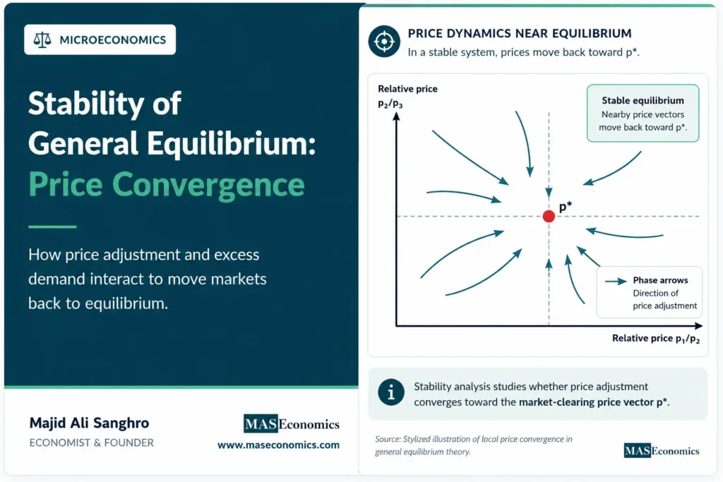
Phase arrows show convergence

A phase-arrow diagram gives a compact way to show price adjustment. In a two-price system, each point represents a combination of relative prices. Arrows show the direction in which prices move under the adjustment rule. Equilibrium is the point where adjustment pressure disappears.

The diagram shows a stable case. Arrows from nearby price vectors point toward \(p^*\). This means that small deviations create price pressures that reduce the deviation rather than enlarge it.

An unstable diagram would look different. Arrows would point away from equilibrium, or they would circle without moving inward. The economic meaning would be that the adjustment rule does not restore market clearing after a disturbance.

Own-price effects are not enough

Single-market intuition often focuses on own-price effects. If the price of a good rises, demand for that good tends to fall and supply tends to rise. In isolation, that creates a stabilizing force. Excess demand falls when price rises, and excess supply falls when price falls.

General equilibrium adds cross-price effects. A rise in one price changes the relative attractiveness of other goods. It changes real income for people who own the more expensive good. It changes production costs for firms that use it as an input. These effects can either reinforce or weaken stability.

For example, if the price of energy rises, excess demand for energy may fall. But the same price change can raise production costs, reduce real wages, shift demand toward substitutes, and change labor-market conditions. The direct stabilizing effect in the energy market may be accompanied by destabilizing effects elsewhere.

This is why stability cannot be inferred from downward-sloping demand curves alone. The full excess demand system matters, including every relevant cross-market response.

Speed can produce overshooting

Even when the direction of adjustment is broadly correct, the speed of adjustment can affect stability. A small response to excess demand may move prices gradually toward equilibrium. A large response may overshoot the equilibrium and create excess supply in the opposite direction.

With one market, overshooting can produce oscillation. A low price creates excess demand, the price rises too much, excess supply appears, the price falls too much, and the pattern repeats. The same logic can occur in many markets, but with more complicated paths because every price movement affects several excess demands.

The parameter \(\lambda\) in the adjustment rule captures this issue:

A larger \(\lambda\) means prices react more aggressively to excess demand. Faster adjustment is not always better. If reactions are too strong relative to the structure of demand and supply, convergence can be replaced by cycles or divergence.

Real markets add further timing complications. Some prices change continuously, while others are set by contracts. Asset prices may adjust quickly. Wages, rents, and regulated prices may adjust slowly. Different speeds across markets can shape the path back toward, or away from, equilibrium.

Walras law limits adjustment

Walras law states that the total value of excess demand across all markets equals zero when budget constraints are respected:

Walras Law

This restriction matters for stability because market imbalances are not independent. Excess demand in one market must be matched by excess supply somewhere else in value terms. Price adjustment therefore moves through a constrained system.

Walras law also implies that one market-clearing equation is redundant when all prices are positive. If all but one market clear, the last market must clear as well. Stability analysis must respect this accounting structure. Treating every market as fully independent can misstate the dynamics.

The law does not guarantee convergence. It only restricts the space in which adjustment occurs. Prices can still move in cycles, diverge, or converge slowly while satisfying the value-balance condition at every point.

Multiple equilibria complicate stability

Stability becomes more subtle when a model has more than one equilibrium. A price vector may converge toward one equilibrium from some starting points and toward another equilibrium from different starting points. The economy’s path can depend on initial conditions.

The set of starting points that converge to a particular equilibrium is called its basin of attraction. Inside that basin, price adjustment pulls the system toward that equilibrium. Outside it, the same adjustment rule may pull the system somewhere else.

This distinction matters because local stability does not imply global stability. An equilibrium may be stable for small disturbances but irrelevant for larger shocks. A price vector far from equilibrium may converge to a different clearing point or fail to converge at all.

In this sense, stability analysis gives a more careful language for equilibrium selection. It asks not only which equilibria exist, but also which ones are reachable under a specified adjustment process.

Real economies add frictions

Theoretical stability analysis often abstracts from institutions to focus on the price system. Real economies include contracts, inventories, credit constraints, search frictions, expectations, and policy rules. These features can strengthen or weaken convergence.

Inventories can stabilize goods markets by absorbing short-run gaps between demand and supply. Credit constraints can destabilize adjustment by forcing agents to cut spending when prices or incomes move against them. Expectations can create self-reinforcing movements if agents buy because they expect prices to rise further.

False trading is another important friction. If trades occur before equilibrium prices are reached, endowments and wealth positions change during the adjustment process. The excess demand system itself can shift while prices are moving.

For this reason, general equilibrium stability is best understood as a benchmark. It identifies the conditions under which price signals can coordinate plans. Real-world analysis then adds the institutions that determine whether this coordination is fast, slow, incomplete, or unstable.

Stability clarifies market coordination

The concept of stability clarifies what equilibrium theory can and cannot claim. A competitive equilibrium is not automatically a prediction. It becomes predictive only if there is a credible process that moves prices and quantities toward it.

Stability also gives meaning to temporary disturbances. If an equilibrium is locally stable, a small shock creates forces that tend to restore the original price vector. If it is unstable, a small shock can push the system toward a different path.

This is why stability matters for comparative statics. A model may show how equilibrium changes after a parameter shifts, but the result is incomplete if the old and new equilibria are not dynamically meaningful. The question is not only where the new equilibrium lies, but whether the price system can plausibly move toward it.

Stability therefore connects formal equilibrium analysis to economic adjustment. It turns market clearing from a static condition into a question about the direction and discipline of price movements.

Explains

Conclusion

Stability of general equilibrium asks whether prices converge toward market-clearing values after a disturbance. It is separate from equilibrium existence, because a price vector can clear markets in theory without being reachable through a given adjustment process.

The main issue is cross-market feedback. In a connected economy, the excess demand for each good depends on many prices, not only its own price. Local stability depends on whether those interactions pull prices back toward equilibrium or push them away.

Stability analysis does not prove that real markets always self-correct. It provides a disciplined way to study when price signals coordinate plans, when adjustment overshoots, and when equilibrium remains only a static solution rather than a dynamic destination.

Frequently Asked Questions

Thanks for reading! If you found this helpful, share it with friends and spread the knowledge. Happy learning with MASEconomics