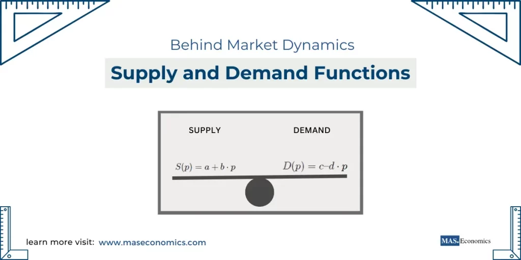
Understanding the supply and demand functions that drive market dynamics and equilibrium is key to analyzing markets effectively. These functions allow economists to quantify how price changes impact quantities demanded and supplied and predict market behavior. In this blog post, we’ll dive into the mathematical structure behind supply and demand functions and how these functions are used to determine market equilibrium.
Rather than focusing purely on economic theory, we will go deeper into the functional form of supply and demand functions, how they are represented and analyzed mathematically, and how they interact to define equilibrium.
The Mathematics of Supply Functions
Understanding the Supply Function
In economics, the supply function is a mathematical representation of the relationship between the price of a good and the quantity supplied. Mathematically, this is often written as:
\( S(p) = a + b \cdot p \)
In this equation, \( S(p) \) represents the quantity of the good supplied at a given price \( p \). The constant \( a \) represents the intercept, indicating the baseline supply level when the price is zero. The coefficient \( b \) reflects the responsiveness of supply to price changes; it shows how much the quantity supplied changes for each unit change in price.
For example, let’s consider the supply function for a commodity like wheat:
\( S(p) = 5 + 2p \)
This function suggests that at a price of zero, there is still a baseline supply of 5 units. As the price increases by one unit, the quantity supplied increases by 2 units. This linear function helps capture the positive relationship between price and quantity supplied, which is consistent with the law of supply—producers are willing to supply more at higher prices.
Individual vs. Aggregate Supply
In macroeconomics, we distinguish between individual supply functions (specific to a single firm or producer) and the aggregate supply function (the total supply of a good or service across the market). In a perfectly competitive market, the marginal cost often coincides with the supply function, reflecting that firms adjust their supply based on marginal profitability.
The aggregate supply function is crucial for understanding the behavior of the overall market. It is influenced by the sum of all individual suppliers and can be affected by changes in factors such as production technology, input costs, and government policies. The aggregate supply function helps economists predict how changes at the macro level (e.g., interest rates or taxes) impact the total quantity of goods supplied in an economy.
Non-Linear Supply Functions
While linear supply functions are often used for simplicity, real-world supply functions can be non-linear. A non-linear supply function may take the form:
\( S(p) = a + bp + cp^2 \)
This type of function suggests that the quantity supplied may increase at an increasing or decreasing rate as the price rises, depending on the sign and magnitude of the \(c \) coefficient. Non-linear supply functions are especially relevant in cases where production costs increase disproportionately as output scales, such as when firms face capacity constraints or diminishing returns to scale.
The Mathematics of Demand Functions
Demand Function Representation
A demand function illustrates how the quantity demanded of a good or service changes in response to its price. Mathematically, the demand function is written as:
\( D(p) = c – d \cdot p \)
In this function, \( D(p) \) represents the quantity of the good demanded at a given price \( p \). The constant \( c \) indicates the intercept, which is the theoretical quantity demanded when the price is zero. The coefficient \( d \) represents how sensitive demand is to price changes, showing the reduction in quantity demanded with each increase in price.
For example, consider the demand function for a product like oranges:
\( D(p) = 30 – 3p \)
This implies that if the price of oranges is zero, the quantity demanded would be 30 units. However, for every unit increase in price, the quantity demanded decreases by 3 units, showing the inverse relationship between price and demand.
Inverse Functions and Their Importance
Sometimes, it is helpful to express price as a function of quantity demanded—this is known as the inverse demand function:
\( p = f^{-1}(D) \)
For example, if we consider \( D(p) = 30 – 3p \), we can rearrange to express price in terms of quantity demanded:
\( p = 10 – \frac{D}{3} \)
This representation is particularly useful when calculating consumer surplus or analyzing the price consumers are willing to pay for a given quantity of goods. It allows for a clearer understanding of how much value consumers place on different quantities of a product.
Non-Linear Demand Functions
Like supply functions, demand functions can also be non-linear. A typical non-linear demand function may look like:
\( D(p) = c – dp + ep^2 \)
Non-linear demand functions may indicate that the impact of price changes on demand varies across different price levels. For instance, certain products might exhibit price insensitivity up to a certain threshold, after which demand changes drastically. Understanding these non-linearities is crucial in determining the optimal pricing strategy for firms.
Market Equilibrium
The equilibrium in a market is found at the price where the quantity supplied equals the quantity demanded. At this point, the market “clears,” meaning there is neither a surplus nor a shortage of the good. Mathematically, equilibrium is determined by setting the supply function equal to the demand function and solving for price \( p\):
\( S(p) = D(p) \)
Consider the functions:
- Supply Function: \( S(p) = 5 + 2p \)
- Demand Function: \( D(p) = 30 – 3p \)
To find the equilibrium price, set \( S(p) \) equal to \( D(p) \):
\( 5 + 2p = 30 – 3p \)
Solving for \( p \):
\( 5p = 25 \implies p = 5 \)
To find the equilibrium quantity, substitute \( p = 5 \) back into either the supply or demand function:
\( S(5) = 5 + 2(5) = 15 \)
Thus, the equilibrium price is $5, and the equilibrium quantity is 15 units.
Interpretation of Market Equilibrium
The equilibrium price and quantity represent the market-clearing outcome—where every unit supplied is purchased, and there are no unsatisfied buyers or unsold goods. It reflects a state of balance where neither suppliers nor consumers have any incentive to change their behavior. Any deviation from this equilibrium, such as a change in supply conditions or shifts in demand, will lead to adjustments in price and quantity as the market attempts to return to equilibrium.
For instance, if the price were set above $5, the quantity supplied would exceed the quantity demanded, leading to a surplus. Producers, in response to accumulating inventories, would likely reduce prices to attract more buyers, eventually bringing the market back to equilibrium. Conversely, if the price were below $5, a shortage would arise, leading to higher prices as consumers compete for the limited goods available.
Shifts in Supply and Demand Functions
When factors other than price affect supply and demand, the entire functions shift. These shifts can be captured mathematically by altering the intercept terms of the supply or demand functions.
Shifting the Supply Function
If there is an advancement in technology that makes production cheaper, the supply function might shift to the right, indicating an increase in supply at every price level. Mathematically, if our original supply function is:
\( S(p) = 5 + 2p \)
An improvement in technology might change it to:
\( S(p) = 10 + 2p \)
This new function suggests a higher quantity supplied at any given price, due to technological efficiency gains. On the other hand, an increase in input costs, such as raw materials or labor, could shift the supply function to the left, decreasing supply at each price level.
Shifting the Demand Function
For the demand function, changes in consumer income or preferences can cause shifts. For instance, if consumers’ income increases, they may be willing to buy more of a product at the same price, shifting the demand curve to the right. If our initial demand function is:
\( D(p) = 30 – 3p \)
An increase in income might change it to:
\( D(p) = 40 – 3p \)
This new function shows increased demand at each price level, indicating higher purchasing power among consumers. Alternatively, a shift in consumer preferences away from a product—perhaps due to changing tastes or the introduction of a superior substitute—would cause the demand function to shift to the left.
Effects of Shifts on Equilibrium
When supply or demand shifts, the equilibrium price and quantity change accordingly. Suppose there is an increase in consumer income that shifts the demand function from \( D(p) = 30 – 3p \) to \( D(p) = 40 – 3p \). To determine the new equilibrium:
Set the supply function equal to the new demand function:
\( 5 + 2p = 40 – 3p \)
Solving for \( p \):
\( 5p = 35 \implies p = 7 \)
Substituting \( p = 7 \) back into the supply function:
\( S(7) = 5 + 2(7) = 19 \)
The new equilibrium price is $7, and the equilibrium quantity is 19 units. This new equilibrium reflects the increased willingness of consumers to purchase more at higher price levels due to their increased income.
Conclusion
Supply and demand functions are at the core of economic analysis, providing a structured approach to understanding the dynamics of markets and equilibrium. By framing supply and demand as mathematical functions, economists can quantify relationships, predict outcomes, and analyze the effects of changes in market conditions.
FAQs:
What is the purpose of supply and demand functions in economics?
Supply and demand functions represent the relationship between price and quantity for goods in a market. They help economists understand how price changes impact the quantity supplied or demanded, predict market behavior, and determine equilibrium where quantity supplied equals quantity demanded.
How is a supply function typically represented?
A supply function is often written as \( Q_s = a + bP \), where \( Q_s \) is the quantity supplied at a given price \( P \). The constant \( a \) indicates baseline supply, and the coefficient \( b \) shows how much quantity supplied changes with each unit increase in price, reflecting the direct relationship between price and supply.
What role does the demand function play in market dynamics?
The demand function represents the inverse relationship between price and quantity demanded, often in the form \( Q_d = c – dP \). It shows how the quantity consumers are willing to purchase changes with price. The demand function helps illustrate consumer behavior, and when combined with the supply function, it determines market equilibrium.
How do you find the market equilibrium using supply and demand functions?
Market equilibrium occurs where quantity supplied equals quantity demanded. To find it, set the supply function equal to the demand function and solve for price. Substitute this price back into either function to find the equilibrium quantity. This gives the price and quantity where the market clears, with no surplus or shortage.
How do shifts in supply or demand affect equilibrium?
Shifts in supply or demand, due to factors like changes in production costs or consumer income, alter the equilibrium. An increase in demand shifts the demand curve right, raising both equilibrium price and quantity. An increase in supply shifts the supply curve right, lowering equilibrium price but increasing quantity.
Thanks for reading! Share this with friends and spread the knowledge if you found it helpful.
Happy learning with MASEconomics


