
Welcome to MASEconomics, your guide to the world of economics. In this blog, we will explore the fundamental concepts of economics, such as supply and demand, equilibrium, and Market Efficiency.
Supply and Demand
Supply and demand are the two most important concepts in economics. They explain how markets work, how prices are set, and how resources are allocated.
To comprehend their significance, let’s break down each concept:
Demand
Consumers Desires
Demand refers to the number of goods or services that buyers are willing and able to purchase at different prices over a certain time period. This is connected to the ‘law of demand’, which says that if the price of a product goes down, the amount that consumers want to buy goes up, assuming all other factors stay the same.
What drives consumer demand? Several factors can influence this, such as personal preferences, income levels, the prices of similar goods (substitutes and complements), consumer expectations, and the makeup of the population. For instance, if the price of a similar good goes down, consumers might change their preferences and want more of that particular good.
Demand Schedule and Curve:
Demand Schedule
Imagine a list that outlines how much a buyer is willing to purchase at different prices. This is precisely what a demanding schedule does. It offers insights into consumers’ preferences, decisions, and responses to price changes.
A demand schedule is a table that shows the quantity of a good that consumers are willing to buy at different prices. It is a useful way to summarize the relationship between price and quantity demanded.
To graphically represent demand, we need a demand curve.
Demand Curve
The demand curve is a graphical representation of the demand schedule. It is a downward-sloping line that shows the inverse relationship between price and quantity demanded. The law of demand states that ceteris paribus, as the price of good decreases, the quantity demanded by consumers will increase.
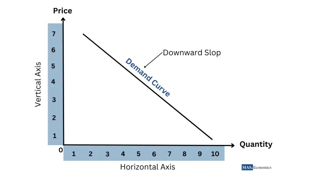
Imagine you’re in the market for cupcakes. A demand schedule might outline how many cupcakes you’re willing to buy at various prices. When this data is plotted on a graph, we create a demand curve. As the price of cupcakes decreases, the quantity you’re willing to purchase increases. The demand curve elegantly visualizes this inverse relationship.
Law of Demand
The Underlying Principle
Central to demand is the Law of Demand, a principle that ceteris paribus, or all else equal, states an intriguing fact: as the price of good decreases, the quantity demanded by consumers increases. This foundational law underscores the intricate dance between consumer behavior and pricing strategies.
The law of demand can be explained by a number of factors, including the income effect, the substitution effect, and the wealth effect.
- The income effect states that when the price of a good decreases, consumers have more money to spend on other goods, so they will buy more of those goods.
- The substitution effect states that when the price of a good decreases, consumers will substitute that good for other goods that have become relatively more expensive.
- The wealth effect states that when the price of a good decreases, consumers feel wealthier, so they are more likely to buy that good and other goods.
Cross Demand, Derived Demand, and Composite Demand
Before we plunge into the core of demand, let’s explore three concepts that set the stage for our exploration: cross-demand, derived demand, and composite demand.
Cross Demand
The demand for a good can be affected by the demand for other goods. This is known as cross-demand. There are two types of cross-demand: complementary goods and substitute goods.
- Complementary goods are goods that are often consumed together. For example, peanut butter and jelly are complementary goods. If the price of peanut butter decreases, the demand for jelly will likely increase. This is because consumers are more likely to buy both goods together when peanut butter is cheaper.
- Substitute goods are goods that can be used in place of each other. For example, coffee and tea are substitute goods. If the price of coffee decreases, the demand for tea will likely decrease. This is because consumers are more likely to buy coffee when it is cheaper.
Derived Demand
Another type of demand is derived demand. This is the demand for a good that is used to produce another good. For example, the demand for steel is derived from the demand for cars. If the demand for cars increases, the demand for steel will also increase. This is because more steel will be needed to produce more cars.
Composite Demand
Finally, there is composite demand. This is the demand for a good that has multiple uses. For example, the demand for milk is affected by the demand for milk products, such as cheese, butter, and yogurt. If the demand for milk products increases, the demand for milk will also increase.
Change in Quantity Demanded vs. Change in Demand
Now, let’s distinguish between two important concepts: change in quantity demanded and change in demand.
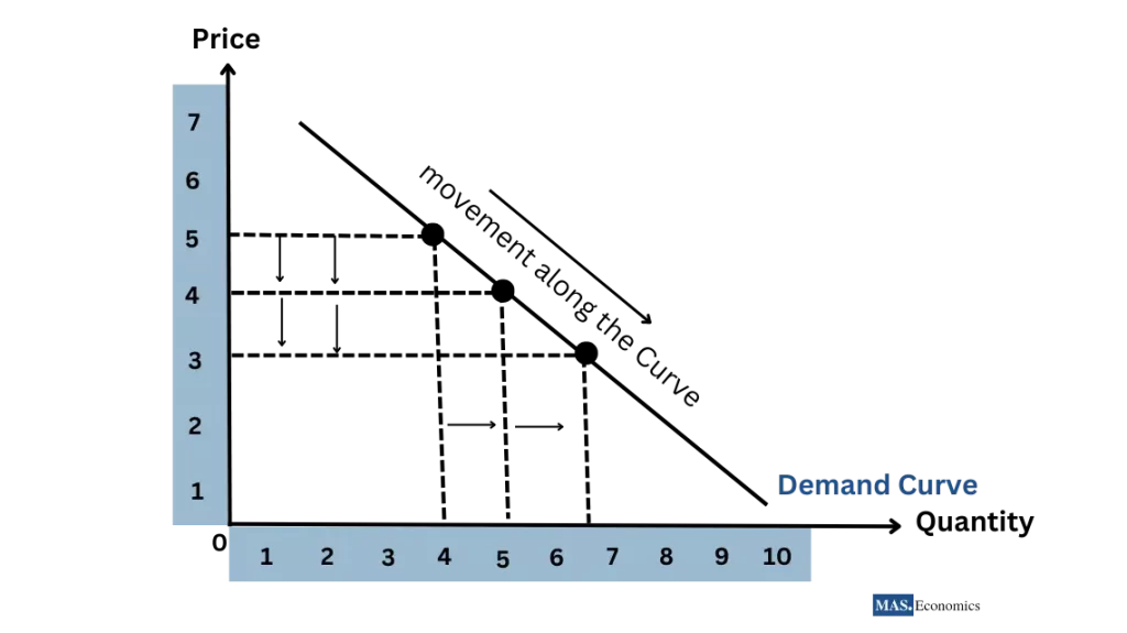
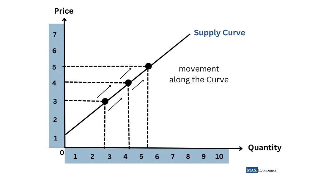
Change in Quantity Demanded: This occurs when the price of good changes, leading to a shift along the existing demand curve. It’s a direct result of price fluctuations and reflects movement along the curve.
Imagine your favorite ice cream’s price drops. As a result, you buy more of it. This change is reflected as movement along the demand curve.
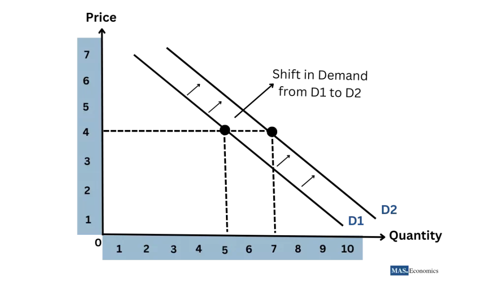
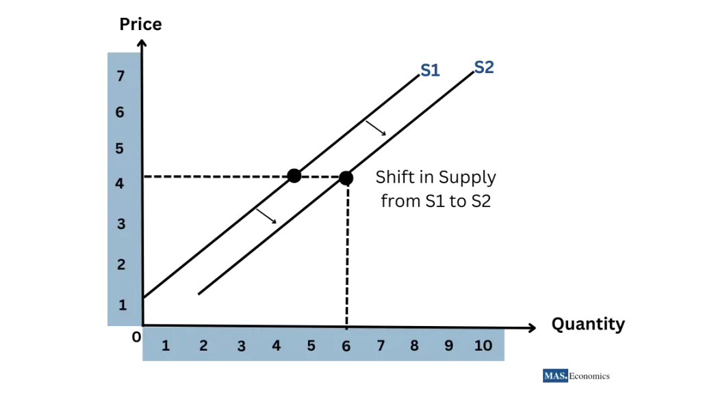
Change in Demand: In contrast, a change in demand refers to shifts in the entire demand curve. It arises from factors other than price, such as shifts in consumer preferences, income levels, or population demographics.
If your income increases, you might decide to buy more luxury goods like high-end electronics. This shift in purchasing behavior is a change in demand, altering the entire demand curve.
Non-Price Determinants of Demand
The Demand Shifters
An integral part of demand analysis is understanding the factors that cause demand to shift. These non-price determinants, or demand shifters, encompass variables beyond price that influence consumer behavior. Let’s explore these determinants in an informative table:
| Determinant | Short Explanation | |
|---|---|---|
| Income | The level of income consumers have affects their purchasing power and ability to buy goods and services. | |
| Consumer Preferences | Individual preferences, tastes, and trends influence what consumers choose to buy. | |
| Price of Related Goods | The prices of substitutes and complements impact the demand for a specific good. | |
| Population Demographics | Factors like age, gender, and location impact the composition of the consumer base and their preferences. | |
| Consumer Expectations | Anticipated changes in future prices, income, or other economic conditions influence current demand decisions. | |

|
||
Let’s now turn our attention to the concept of supply. Just as understanding consumer behavior is crucial for comprehending demand, exploring the behavior of producers and the factors influencing supply is essential to complete the picture of market interactions.
Supply
Producers Offerings
Supply is the amount of a good or service that producers are willing and able to sell at different prices over a certain time period. The law of supply states that, ceteris paribus, as the price of goods increases, the quantity supplied by producers will also increase.
The factors that can affect supply include:
- Cost of production: The higher the cost of production, the lower the supply.
- Price of other goods: If the price of a related good increases, the supply of the first good may decrease.
- Technology: New technologies can make it cheaper to produce goods, increasing supply.
- Government policies: Government policies, such as taxes and subsidies, can affect supply.
- Expectations about future prices: If producers expect the price of a good to increase in the future, they may supply less of the good today.
Supply Schedule and Curve
The supply schedule is a table that shows the quantity of a good that producers are willing to supply at different prices.
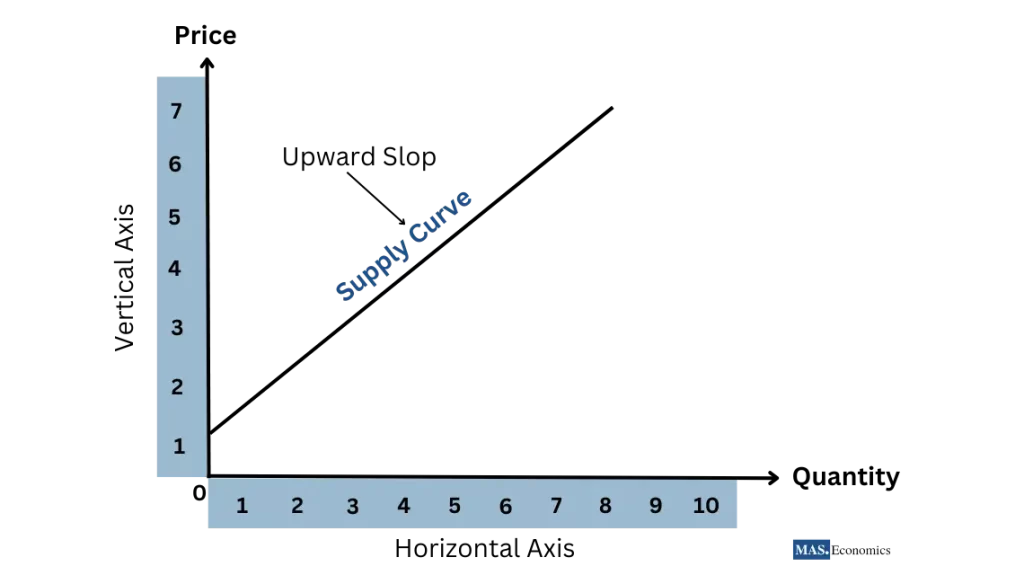
The supply curve is a graphical representation of the supply schedule. It is an upward-sloping line that shows the positive relationship between price and quantity supplied.
Law of Supply
The Law of Supply states that ceteris paribus, there is a direct relationship between the price of a product and the quantity supplied by producers. As prices increase, the quantity supplied tends to increase, and vice versa.
Exceptional Supply and Joint Supply
While examining supply, it’s crucial to delve into exceptional supply and joint supply, adding further layers of complexity to the concept.
Exceptional Supply
Exceptional supply occurs when the usual supply behavior is reversed. Typically, when prices increase, so does the quantity supplied. However, in exceptional supply, this isn’t always the case.
For example, during an agricultural crisis like a drought or pest invasion, even if prices go up, the supply might decrease because crops can’t grow. This situation defies the commonly known positive relationship between price and supply.
Joint Supply
Joint supply occurs when producing one good automatically results in the production of another. For example, cattle farming produces both meat and leather. These are joint products because they come from the same source – the cow. The supply of these joint products is interconnected, meaning changes in the production of one will affect the other.
For example, if the price of meat increases, farmers may be more likely to produce more cattle. This will lead to an increase in the supply of leather, even though the price of leather has not changed.
Change in Quantity Supply vs Change in Supply
A change in quantity supplied refers to a movement along the supply curve due to a change in the price of the good itself. On the other hand, a change in supply occurs when any factor other than the price of the good changes, leading to a shift in the entire supply curve.
Non-Price Determinants of Supply
Here are the non-price determinants of supply, factors that can influence the quantity of a good that producers are willing to supply at a given price. These factors can cause the entire supply curve to shift:
| Determinant | Explanation | Example |
|---|---|---|
| Resource Prices | The cost of inputs used in production influences supply. Higher resource prices can decrease supply, while lower prices may enhance it. | If the price of crude oil increases, the supply of gasoline might decrease due to higher production costs. |
| Technology | Technological advancements improve efficiency, leading to increased supply. | Introduction of advanced machinery in automobile manufacturing raises supply due to enhanced productivity. |
| Number of Sellers | The quantity supplied can shift with changes in the number of producers in the market. | If new firms enter the smartphone market, the overall supply of smartphones may rise. |
| Producer Expectations | Producers’ anticipations about future conditions can influence their current supply decisions. | If coffee producers expect a drought next year, they might reduce current supply to preserve resources. |
| Government Policies | Government regulations, taxes, and subsidies shape production costs and supply choices. | A tax incentive for renewable energy might boost the supply of solar panels. |
|
|
||
Now, let’s delve into market equilibrium, where supply and demand find their balance, shaping resource allocation and pricing dynamics.
Equilibrium
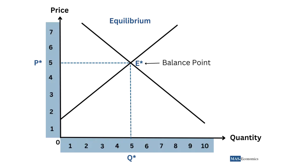
Supply and demand are two fundamental economic forces that interact to establish the equilibrium price and quantity in a market.
The equilibrium, or balance point, is reached when the amount of a good or service that producers are willing to supply matches the amount that consumers are willing to buy. This equilibrium price symbolizes a consensus between buyers and sellers on the worth of a good or service.
However, market equilibrium is not a fixed state. It is a dynamic process shaped by continuous adjustments in supply and demand.
Let’s break this down further:
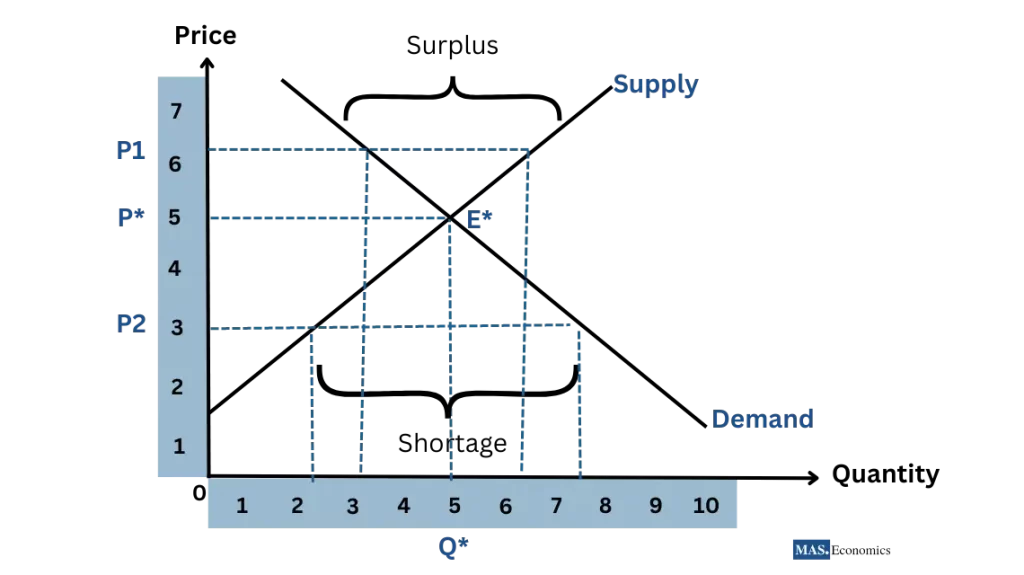
- Excess demand occurs when the price is less than the equilibrium price. In this scenario, consumers want to buy more of the good or service than producers are willing to sell. This creates a shortage.
- Excess supply occurs when the price is greater than the equilibrium price. In this scenario, producers want to sell more than consumers want to buy. This results in a surplus.
Change in Equilibrium and Output
The equilibrium price and quantity can change due to changes in demand, supply, or both.
- Change in Demand: If demand increases, the equilibrium price and quantity rise. This is because when demand increases, there are more buyers who want to buy the good or service at any given price. This drives up the price and also leads to an increase in the quantity supplied.
- Change in Supply: An increase in supply leads to a lower equilibrium price but a higher equilibrium quantity. This is because when supply increases, there are more sellers who want to sell the good or service at any given price. This drives down the price and also leads to an increase in the quantity demanded.
- Change in Both Demand and Supply: The combined effect of changes in demand and supply can lead to varied outcomes, affecting both equilibrium price and quantity. For example, if demand increases and supply decreases, the equilibrium price will rise and the equilibrium quantity will fall.
Market forces have a natural tendency to correct these imbalances. If there’s a surplus, producers may lower their prices to sell their excess goods, bringing the price down towards equilibrium. If there’s a shortage, the high demand may encourage producers to supply more, or it may cause prices to increase, both of which push the price back toward equilibrium.
Determination of Equilibrium
Market equilibrium is achieved through a dynamic process where buyers and sellers interact. When quantity demanded equals quantity supplied, an equilibrium price emerges, signaling the prevailing market rate.
Market Efficiency
Market equilibrium is a state of balance where the quantity of goods supplied equals the quantity of goods demanded. This perfect balance signifies economic efficiency, which is an optimal distribution of resources. In this state, there is neither excess supply (surplus) nor excess demand (shortage). This optimal allocation of resources ensures maximum welfare for both consumers and producers.
Consumer and Producer Surplus
Consumer surplus
Consumer surplus refers to the benefit enjoyed by consumers who were willing to pay a higher price than they had to for a good.
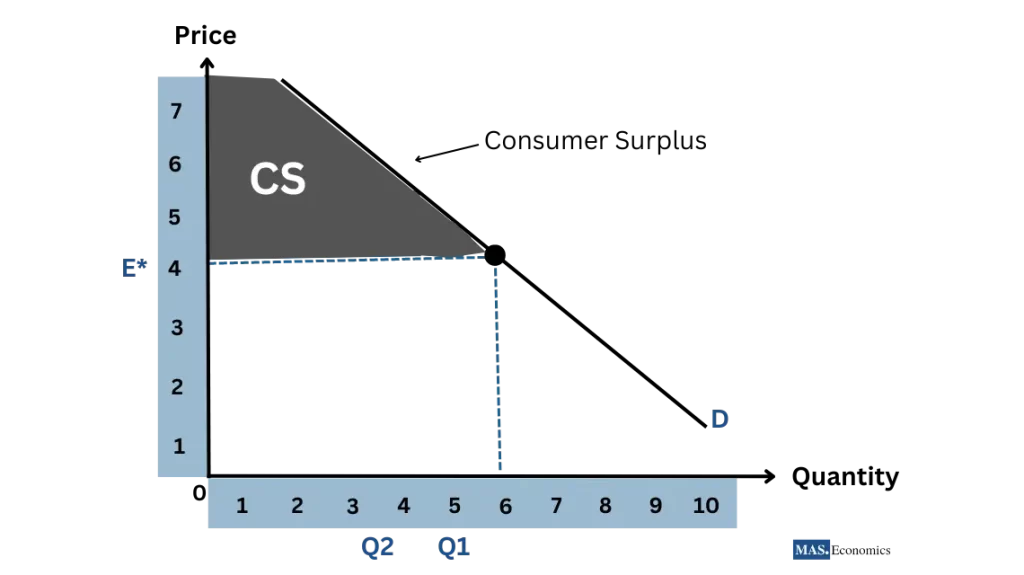
Graphically, it is the area below the demand curve and above the equilibrium price. This is because some consumers are willing to pay more for the good than the equilibrium price. The consumer surplus is a measure of the economic well-being of consumers.
Producer surplus
Producer surplus refers to the benefit enjoyed by producers who would have been willing to sell their product at a lower price than they were able to.
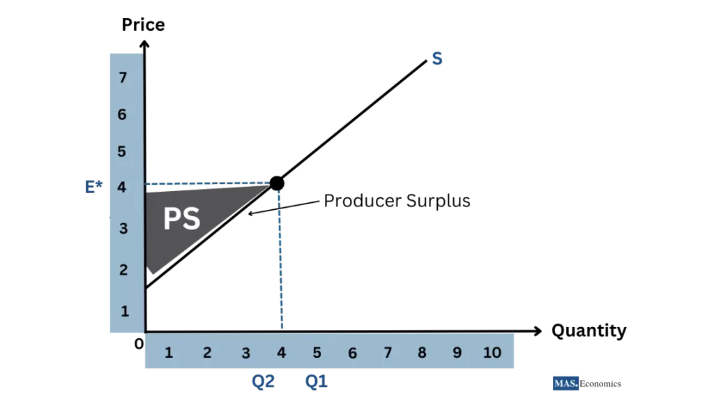
Graphically, it is the area above the supply curve and below the equilibrium price. This is because some producers are willing to sell their products for less than the equilibrium price. The producer surplus is a measure of the economic well-being of producers.
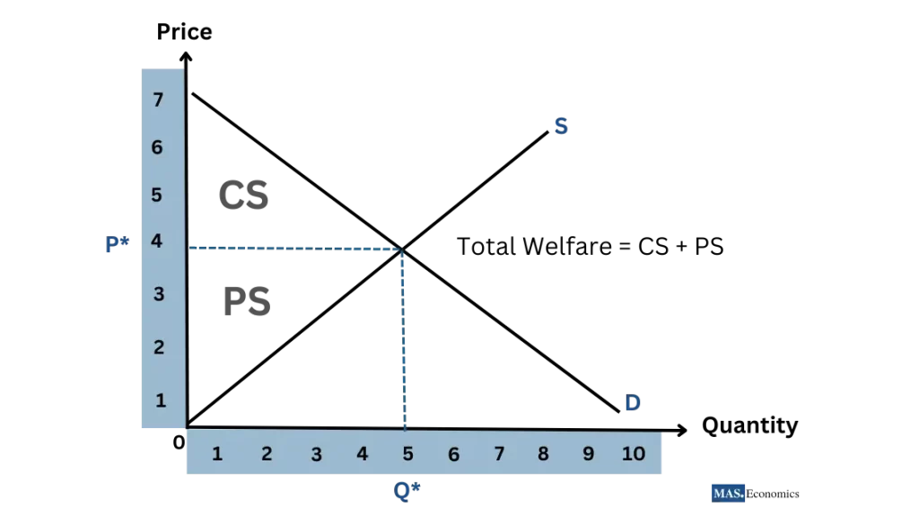
Total Welfare
Total welfare is the sum of consumer surplus and producer surplus. Total welfare is maximized when a market is in equilibrium. Any other price/quantity combination will reduce the sum of consumer and producer surplus and lead to a loss of total welfare.
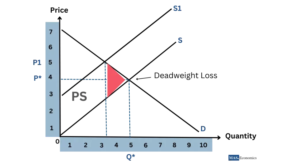
Deadweight Loss
Deadweight loss is the loss of total welfare caused by market inefficiency. It occurs when the market is not in equilibrium, either because of a shortage or a surplus. Deadweight loss is represented by the area between the demand curve and the supply curve, below the equilibrium price.
Thanks for reading! Get ready for our next blog on the concept of elasticities, which will help you understand how consumers and producers respond to changes in the market.
If you enjoyed this series, spread the knowledge by sharing it with friends and on social media.
Happy learning with MASEconomics!