Why do some stocks earn higher returns than others? Is it luck? Skill? Or something more systematic?
Put yourself in the position of an investor in the early 1960s. You know that riskier investments should offer higher returns. That was just common sense. But how much higher? How do you measure risk in the first place? And if you are evaluating a fund manager, how do you know whether their returns come from genuine skill or simply from taking more risk than the market?
These questions plagued finance for decades. Then, in a remarkable burst of intellectual creativity between 1961 and 1966, four economists working independently provided answers that would revolutionize investing. Their model, the Capital Asset Pricing Model, or CAPM, became one of the most influential ideas in financial economics.
The Before CAPM: Risk Without a Price
To appreciate CAPM’s breakthrough, we need to understand the state of finance before the 1960s.
Investors understood intuitively that risk mattered. A government bond was safer than a railroad stock, so the stock should offer higher expected returns. But there was no way to quantify this relationship. How much higher should the return be? Twice as high? Ten times? Nobody knew.
Harry Markowitz had laid the groundwork in 1952 with his portfolio theory. He showed how investors could construct efficient portfolios, those offering the highest expected return for a given level of risk. But Markowitz’s model was normative: it told investors what they should do. It did not explain how assets were actually priced in the market.
What was missing was a bridge from individual investor behavior to market-wide equilibrium. That bridge would be built by four men, working on three continents, largely unaware of each other’s efforts.
The Four Minds Behind CAPM
Jack Treynor (1961)
Jack Treynor, a consultant at Arthur D. Little, wrote an unpublished manuscript in 1961 that contained the essential ideas of CAPM. Though never formally published, his paper circulated among academics and influenced the development of the model. Treynor showed that in equilibrium, the risk premium for any asset should be proportional to its covariance with the market portfolio, a revolutionary insight.
William Sharpe (1964)
A young economist at the University of Washington, William Sharpe, published “Capital Asset Prices: A Theory of Market Equilibrium Under Conditions of Risk” in the Journal of Finance in 1964. His paper provided the clearest and most accessible formulation of the model, complete with the elegant graphical representation that would become standard in textbooks. Sharpe would later win the Nobel Prize in 1990 for this work.
John Lintner (1965)
At Harvard Business School, John Lintner independently developed essentially the same model, publishing his version in the Review of Economics and Statistics in 1965. His paper was more mathematically rigorous than Sharpe’s and explored deeper implications for corporate finance and capital budgeting.
Jan Mossin (1966)
A Norwegian economist, Jan Mossin, published the third independent derivation in Econometrica in 1966. His approach was perhaps the most elegant mathematically, showing how the model emerged naturally from general equilibrium conditions.
The fact that four researchers, working independently, arrived at virtually identical conclusions tells us something: the time was right for a new way of thinking about risk and return.
The Core Idea: Two Prices
CAPM begins with a simple but powerful insight: the market offers investors two prices.
The first is the price of time, the return you can earn without taking any risk. This is the risk-free rate, typically approximated by government bond yields. If you invest in risk-free assets, you earn this rate, no more, no less.
The second is the price of risk, the additional return you can expect for bearing risk. In equilibrium, the market establishes a single price for risk that applies to all assets. Investors can then choose how much risk to bear, and they will be compensated accordingly.
As Sharpe put it in his 1964 paper, in equilibrium, “capital asset prices have adjusted so that the investor, if he follows rational procedures (primarily diversification), is able to attain any desired point along a capital market line.”
Diversification and Systematic Risk
To understand CAPM, we must first understand a crucial distinction: not all risk is created equal.
Consider an investment in a single stock, say, Pakistan State Oil (PSO). Its price fluctuates for many reasons. Some are specific to PSO: a refinery outage, a change in management, a new contract. Other reasons affect the entire market: interest rate changes, economic growth news, and political developments.
Now consider what happens when you diversify by buying 30 or 40 Pakistani stocks. What happens to your risk? The company-specific fluctuations tend to cancel out. When PSO has bad news, maybe another stock has good news. Your portfolio’s overall volatility declines.
But can you eliminate all risk? No. No matter how many Pakistani stocks you buy, you cannot escape the risk that affects the entire Pakistani market, the risk of a recession, a currency crisis, or a change in economic policy. This remaining risk is called systematic risk or market risk.
CAPM’s central insight is this: investors are only rewarded for bearing systematic risk. The risk that can be diversified away, called unsystematic risk, should not earn a premium because investors can eliminate it simply by diversifying.
This seems obvious in hindsight, but it was revolutionary at the time. It meant that a stock’s total volatility (its standard deviation) was not the right measure of its riskiness for pricing purposes. What mattered was its sensitivity to the market.
Beta: The Heart of CAPM
This sensitivity is captured by a single number: beta (\( \beta \)).
Beta measures how much a stock’s returns tend to move with the market. Formally:
Where:
\( R_i \) — the return of stock i
\( R_M \) — the return of the market portfolio
In plain language, beta tells us:
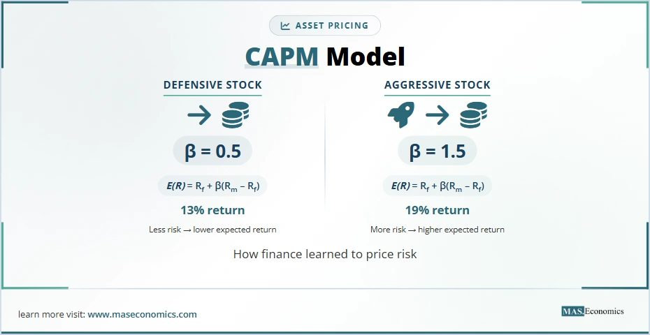
\( \beta = 1 \): The stock moves in lockstep with the market. If the market rises 10%, the stock tends to rise 10%.
\( \beta > 1 \): The stock is more volatile than the market. If \( \beta = 1.5 \), a 10% market rise tends to produce a 15% rise in the stock.
\( \beta < 1 \): The stock is less volatile than the market. If \( \beta = 0.5 \), a 10% market rise tends to produce a 5% rise.
\( \beta = 0 \): The stock has no correlation with the market. Its returns are independent.
A MASEconomics Example
Consider two Pakistani companies:
- Oil and Gas Development Company (OGDC) – a large, established energy company. Its fortunes are tied to global oil prices and the Pakistani economy. Let’s say its beta is 1.2.
- A small textile exporter – its business depends on international demand and cotton prices, which may not move perfectly with the Pakistani stock market. Its beta might be 0.8.
CAPM predicts that OGDC should have a higher expected return than the textile company because it carries more systematic risk. The textile company’s higher total risk (maybe it’s quite volatile) doesn’t matter for pricing because much of that risk is diversifiable.
The CAPM Formula
With beta defined, CAPM gives us a simple linear relationship:
Where:
\( E(R_i) \) – the expected return of stock i
\( R_f \) – the risk-free rate
\( E(R_M) \) – the expected return of the market portfolio
\( [E(R_M) – R_f] \) – the market risk premium
This is the Security Market Line (SML). It says that an asset’s expected return equals the risk-free rate plus a risk premium proportional to its beta.
A Numerical Example
Let’s make this concrete with numbers a Pakistani investor might recognize:
- Risk-free rate (say, 6-month Treasury bill): 10% (this is illustrative, not current)
- Expected market return (KSE-100 index): 16%
- Market risk premium: 6%
Now consider three stocks:
| Stock | Beta | CAPM Expected Return | Calculation |
|---|---|---|---|
| Defensive Ltd. | 0.5 | 13% | \( 10\% + 0.5 \times 6\% \) |
| Market Co. | 1.0 | 16% | \( 10\% + 1.0 \times 6\% \) |
| Aggressive Inc. | 1.5 | 19% | \( 10\% + 1.5 \times 6\% \) |

|
|||
The defensive stock offers a lower expected return (13%) than the market, but also lower risk. The aggressive stock offers a higher expected return (19%) but with greater risk. Investors can choose their position along this line based on their risk tolerance.
The Security Market Line Graphically
Sharpe’s 1964 paper included a now-famous diagram. The Security Market Line plots expected return against beta:

All assets should plot on this line in equilibrium. If an asset plots above the line, it offers too high a return for its beta investors to buy it, driving its price up and its expected return down until it falls back to the line. If an asset plots below the line, investors will sell it, driving its price down and expected return up.
What CAPM Gave the World
CAPM’s elegance and simplicity made it enormously influential. It provided:
1. A Cost of Equity
Companies could now estimate their cost of equity capital. If a firm’s beta was 1.2, the risk-free rate 10%, and the market risk premium 6%, its cost of equity was 17.2% (10% + 1.2 × 6%). This became essential for capital budgeting decisions.
2. A Way to Evaluate Fund Managers
If a mutual fund earned 20% when the market returned 16% and the risk-free rate was 10%, was the manager skilled? CAPM provided an answer. First, calculate the fund’s beta. Suppose it was 1.2. Its expected return was 17.2%. The extra 2.8% (20% – 17.2%) was alpha (\( \alpha \)) the return attributable to manager skill rather than risk-taking.
Positive alpha suggests skill; negative alpha suggests poor performance. This became the standard for evaluating professional investors.
3. A Framework for Thinking About Risk
CAPM shifted the conversation from “how risky is this stock?” to “how does this stock co-vary with the market?” This was a profound conceptual advance.
Why CAPM Might Not Work
For all its elegance, CAPM rests on assumptions that are clearly unrealistic:
Unrealistic Assumptions
- Investors can borrow and lend at the same risk-free rate
- All investors have the same expectations (homogeneous expectations)
- No taxes, no transaction costs
- All assets are publicly traded
- Investors care only about the mean and variance of returns
In the real world, these assumptions don’t hold. Borrowing rates exceed lending rates. Investors have different information and beliefs. Taxes matter. Some assets (human capital, private businesses) aren’t traded.
The Roll Critique
In 1977, Richard Roll delivered a devastating critique: CAPM is untestable because the true market portfolio, which should include all assets, not just stocks, is unobservable. Every test of CAPM is really a joint test of the model and the proxy used for the market. If the model fails, maybe it’s because we used the wrong market proxy.
The Empirical Evidence
When researchers tested CAPM, they found mixed results. The model seemed to work reasonably well for some periods but not others. More troubling, other factors seemed to explain returns better than beta alone.
The Fama-French Three-Factor Model
The most famous challenge to CAPM came from Eugene Fama and Kenneth French in a series of papers beginning in 1992. They found that two additional factors, size and value, had significant power to explain stock returns.
The Size Effect (SMB)
Fama and French observed that small-company stocks tended to outperform large-company stocks, even after adjusting for beta. This became known as the size effect. They created a factor called SMB (Small Minus Big), the return of a portfolio of small stocks minus the return of a portfolio of big stocks.
The Value Effect (HML)
They also found that stocks with high book-to-market ratios (value stocks) tended to outperform stocks with low book-to-market ratios (growth stocks). This became the value effect. They created a factor called HML (High Minus Low), the return of a portfolio of high book-to-market stocks minus the return of a portfolio of low book-to-market stocks.
The Three-Factor Model
Fama and French proposed an expanded model:
Where:
\( s_i \) – measures the stock’s sensitivity to the size factor
\( h_i \) – measures its sensitivity to the value factor
This model explained much more of the variation in stock returns than CAPM alone. Studies on markets around the world, including emerging markets like Turkey and Malaysia, found support for the three-factor model, though results varied.
Evidence from Istanbul
A 2013 study by Veysel Eraslan tested the three-factor model on the Istanbul Stock Exchange from 2003 to 2010. The findings were instructive:
- Market risk factor was effective for all portfolios
- The size factor helped explain returns for small and medium-sized firms, but not for large firms
- Value factor helped explain returns for high book-to-market portfolios
- The model worked, but its power was “not strong and wide.”
This pattern, the model works, but imperfectly, is typical of empirical tests across markets.
A Malaysian Perspective on Sharia-Compliant Stocks
Research on the Malaysian market examined whether the three-factor model applied to Sharia-compliant stocks. These stocks, which meet Islamic religious requirements, might behave differently from conventional stocks. The results generally supported the model’s applicability, suggesting that size and value effects exist even in this specialized segment.
Modern Extensions and Continuing Debates
CAPM and its descendants remain active areas of research. Some key developments:
The Fama-French Five-Factor Model
Fama and French later added two more factors, profitability and investment, creating a five-factor model that explains even more of the variation in returns.
The Carhart Four-Factor Model
Mark Carhart added a momentum factor to the three-factor model, capturing the tendency of stocks that performed well recently to continue performing well.
The Q-Factor Model
More recent work by Hou, Xue, and Zhang proposes a model based on investment and profitability factors derived from corporate finance theory.
Does CAPM Still Matter?
After all these critiques and extensions, you might wonder: should we still teach CAPM? Absolutely.
As a Foundation
Every multi-factor model builds on CAPM’s insights. The idea that assets should be priced relative to systematic risk factors is CAPM’s lasting legacy.
As a Benchmark
CAPM provides a simple, intuitive benchmark. When evaluating a fund manager, the first question is still: “What was their beta, and what alpha did they generate relative to CAPM?”
As a Teaching Tool
CAPM’s elegance makes it the perfect introduction to asset pricing. Students can grasp the intuition before moving on to more complex models.
As a Reminder
CAPM reminds us that not all risk is priced. Diversifiable risk doesn’t earn a premium. This fundamental insight shapes how we think about everything from portfolio construction to corporate finance.
The Bottom Line
The Capital Asset Pricing Model emerged from a remarkable moment in intellectual history, four minds, working independently, converging on the same elegant solution to a pressing problem. It taught us that risk has a price, that only systematic risk matters, and that expected returns are linear in beta.
The model’s assumptions are unrealistic. Its empirical performance is mixed. It has been extended, modified, and in some ways superseded. But it remains the starting point for anyone who wants to understand how financial markets price risk.
And that’s a legacy worth celebrating.
Did you find this article helpful? Share it with someone who loves economics. And remember, at MASEconomics, we make complex ideas simple.