In March 2026, the Bank of Japan held its policy rate at 0.75%, the highest level since 1995. For most central banks, that figure would count as deeply accommodative. For the BoJ, it was the cautious culmination of a quarter‑century journey out of near‑zero rates, a journey that ended negative interest rates only in March 2024 and that is still being calibrated against fragile inflation expectations and a yen carry trade unwinding across global markets. The Federal Reserve sits at 3.50%–3.75% after six cuts, the European Central Bank holds its deposit rate at 2.00%, and economists inside both institutions openly debate how much room remains to cut before policy bumps against the floor again. This is the world that liquidity trap economics describes: a world where the short‑term nominal interest rate, the textbook tool of monetary policy, runs out of room and stops doing the work it is supposed to do.
After the 2008 financial crisis pinned the Fed at zero for seven years, after the eurozone spent nearly a decade with negative deposit rates, and after the post‑pandemic inflation surge offered a brief escape that may not last, the liquidity trap has become a defining structural problem of monetary policy in advanced economies. The conditions that produce it have become persistent features of low‑growth, high‑debt, demographically aging economies.
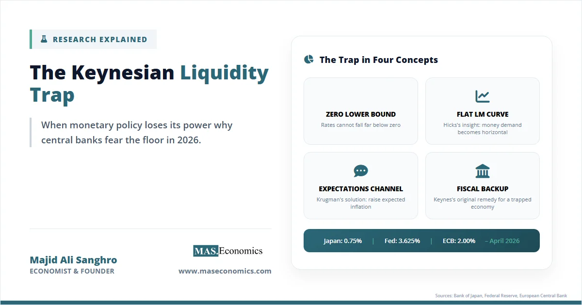
Liquidity Trap: Core Idea
The liquidity trap was John Maynard Keynes’s answer to an anomaly that classical economics could not handle. In The General Theory of Employment, Interest and Money (1936), Keynes argued that at sufficiently low interest rates, the demand for money becomes perfectly elastic. Households and firms hold any additional liquidity the central bank injects rather than spending it or lending it out. The reasoning is straightforward: when interest rates are very low, bonds offer almost no yield over cash, and the risk of capital loss from any future rate increase looms large. Money and bonds become near-perfect substitutes, and pumping more reserves into the system simply swells idle balances.
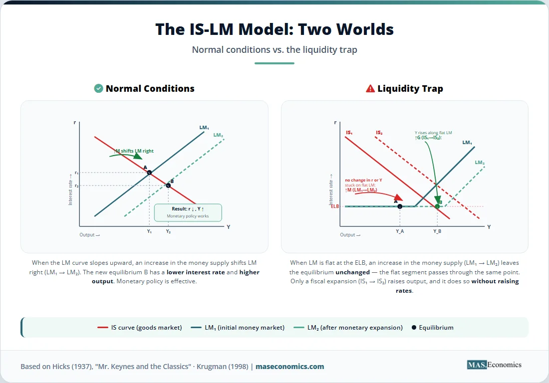
John Hicks formalised the idea four years later in his 1937 paper “Mr. Keynes and the Classics,” which gave us the IS-LM diagram still taught today. In Hicks’s representation, the LM curve, which traces equilibria in the money market, becomes flat at very low interest rates. Once the economy enters that flat region, shifting the LM curve outward through monetary expansion no longer reduces the equilibrium interest rate, because the rate cannot fall further. The IS curve does the rest of the work, but it is the IS curve that determines output, and the central bank has no direct lever on it. Monetary policy is, in Hicks’s phrase, pushing on a string. For a more detailed treatment of the underlying mechanics, our article on the IS-LM framework walks through the algebra and policy implications step by step.
Modern macroeconomics restated the problem in slightly different language. Because nominal interest rates on bank reserves and short-term bonds cannot fall significantly below zero without triggering large-scale conversion to physical cash, there is a floor, the zero lower bound (ZLB), or, allowing for the modest costs of holding cash, the effective lower bound (ELB). When a negative output gap and below-target inflation call for a real interest rate that requires a deeply negative nominal rate, conventional policy hits the wall. The trap is therefore not a quirk of money demand alone but a binding constraint on the central bank’s ability to deliver the real interest rate the economy needs. Paul Krugman’s 1998 paper “It’s Baaack: Japan’s Slump and the Return of the Liquidity Trap,” published in the Brookings Papers on Economic Activity, was the work that pulled the concept back from the textbook margins and showed it was alive in the data.
The clearest definition is therefore the one most useful for policy: a liquidity trap is the state in which the policy rate cannot be cut far enough to restore aggregate demand, because further cuts would either be technically impossible, prohibitively costly to the banking system, or impossible to commit to credibly. Everything that central banks did after 2008, from quantitative easing to forward guidance to negative deposit rates, was an attempt to escape that constraint without lowering the policy rate further.
Liquidity Trap Mathematics
The textbook IS-LM presentation captures the trap in two equations. The IS curve relates real output \( Y \) to the real interest rate \( r \) through the goods market:
where \( C \) is consumption, \( I \) investment, \( T \) taxes, \( G \) government spending, and \( NX \) net exports. Investment depends inversely on the real interest rate, so the IS curve slopes downward in \( (Y, r) \) space. The LM curve relates the real money supply \( M/P \) to output and the nominal interest rate \( i \) through money market equilibrium:
with money demand \( L \) increasing in \( Y \) and decreasing in \( i \). In normal conditions, \( L \) is well-behaved and the LM curve slopes upward. But Keynes’s insight was that as \( i \to i_{\min} \), the partial derivative \( \partial L / \partial i \to -\infty \). Money demand becomes perfectly elastic. The LM curve flattens, and an outward shift in \( M/P \) no longer moves the equilibrium output.
The modern reformulation uses the Euler equation from a representative-agent model. In the version Krugman developed for Japan, the consumption Euler equation links current consumption \( C_t \), expected future consumption \( C_{t+1} \), the nominal interest rate \( i_t \), and expected inflation \( \pi^e_{t+1} \):
where \( \beta \) is the discount factor. Rearranging gives the real rate \( r_t = i_t – \pi^e_{t+1} \) needed to clear the goods market. If the natural real rate \( r^* \) (the rate consistent with full employment and on-target inflation) is, say, \( -2\% \), and expected inflation is \( 0\% \), then the required nominal rate is \( -2\% \). If the ELB is \( i_{\min} \approx 0 \), the gap \( i_{\min} – r^* – \pi^e = 2\% \) is the deflationary shortfall the economy cannot close through conventional rate cuts.
Krugman’s key contribution was showing that escape requires changing \( \pi^e \). If the central bank can credibly commit to higher future inflation, it lowers the real rate today even with the nominal rate stuck at zero. The problem is credibility: a central bank that has spent decades fighting inflation must somehow promise it will tolerate inflation later, and rational agents may refuse to believe the promise. This is the liquidity trap not as a mechanical floor but as a credibility problem.
| Variable | Meaning | Role in the Trap |
|---|---|---|
| \( i_t \) | Nominal policy rate | Cannot fall meaningfully below \( i_{\min} \) |
| \( r_t \) | Real interest rate (\( i_t – \pi^e_{t+1} \)) | What investment and consumption respond to |
| \( r^* \) | Natural / neutral real rate | Rate consistent with full employment |
| \( \pi^e_{t+1} \) | Expected inflation | Only lever left when \( i_t \) is stuck |
| \( i_{\min} \) | Effective lower bound (ELB) | Floor set by cash storage costs and bank profitability |
| \( L(i, Y) \) | Money demand function | Becomes perfectly elastic near \( i_{\min} \) |
| \( \beta \) | Discount factor | Governs intertemporal substitution in the Euler equation |
 | ||
Table 1. Variables in the liquidity trap framework: From IS-LM to the modern Euler equation.
Assumptions of Liquidity Traps
The textbook trap rests on several assumptions that have aged unevenly. The first is that the lower bound is exactly zero. Cash dominates any negative-yielding asset because storing cash, while not free, costs less than a sufficiently negative interest rate. In practice, the ECB held its deposit facility rate at \( -0.50\% \) from September 2019 to July 2022, the Swiss National Bank reached \( -0.75\% \), and Denmark went to \( -0.75\% \) as well. The sky did not fall. Banks absorbed the costs, partly by exempting tiers of reserves from the negative rate, and the financial system continued to function. The lesson was that the lower bound is closer to \( -0.75\% \) or \( -1.00\% \) than to zero, but it is still bounded. Real rates of \( -3\% \) or \( -4\% \) remain out of reach.
The second assumption is that money demand becomes perfectly elastic at the bound. This was always a strong claim. Empirically, money demand functions estimated for Japan, the US, and the eurozone during their respective ZLB episodes did not show a true horizontal segment. They showed a steepening, not a flattening, of the relationship. The trap operates more through the constraint on the policy rate than through a literal collapse of money demand.
The third assumption, often left implicit, is that no other tool can substitute. Quantitative easing, the large-scale purchase of long-duration assets, was designed precisely to bypass the constraint by acting on long-term yields and term premia rather than the policy rate. Our explainer on quantitative easing covers the mechanics in detail. Whether QE actually escapes the trap or merely reshuffles portfolios is a question economists have argued for fifteen years, but at minimum, it provided central banks with an additional lever during the 2008–2021 period. Forward guidance, exchange rate manipulation through the Mundell-Fleming channel covered in our piece on the Mundell-Fleming model, and outright fiscal coordination all sit outside the canonical IS-LM trap and complicate any simple statement that monetary policy has been disarmed.
The fourth assumption is that fiscal policy is unavailable or refuses to act. Keynes himself thought the trap was a case where fiscal policy ought to take over, because the multiplier on government spending is largest precisely when the central bank cannot crowd it out through higher rates. Modern New Keynesian models confirm that result. The trap is therefore less a failure of macroeconomic policy in general than a failure of the specific arrangement in which monetary authorities are independent and active while fiscal authorities are constrained by debt rules and political deadlock. The post-2008 experience of slow fiscal response, particularly in the eurozone, was a policy choice, not an iron law.
Finally, the trap, as classically described, assumed closed economies and fixed expectations. Open-economy considerations matter because a country in a liquidity trap can still depreciate its currency to import demand from abroad. Expectations matter because, as Krugman showed, the real bite of the trap is whether the central bank can shift \( \pi^e \) upward. Modern central banks at the ELB therefore spend most of their effort on communication, on what they signal about future policy, rather than on the policy rate itself.
Empirical Evidence
Three episodes anchor the empirical literature. Japan reached zero rates in February 1999 and, with the brief exception of 2006–2008, has lived near or below zero for more than a quarter-century. The Bank of Japan introduced quantitative easing in 2001, ended it, reintroduced it in 2013 under Haruhiko Kuroda’s Quantitative and Qualitative Monetary Easing programme, added negative rates in 2016, and only began normalising in March 2024. As of March 2026 the policy rate stands at 0.75%, the highest since 1995, and BoJ board member Hajime Takata has publicly argued that the price stability target is “almost achieved.” Yet the central bank still holds roughly 49% of all outstanding Japanese government bonds, and unwinding that position without breaking the market is a problem with no historical precedent.
The United States hit the ZLB in December 2008 and stayed there until December 2015, then again from March 2020 to March 2022. The Fed conducted three rounds of QE, expanded its balance sheet from under $1 trillion to $4.5 trillion by 2014, and used forward guidance to extend the expected duration of zero rates. Empirical work by Engen, Laubach and Reifschneider (Fed, 2015) estimated that the combination of QE and forward guidance lowered the unemployment rate by about 1.2 percentage points at peak effect. That is meaningful but smaller than what conventional rate cuts of equivalent ambition would have delivered, which is the empirical signature of a binding trap.
The eurozone reached its first ZLB episode after the 2011 sovereign debt crisis. The ECB cut its main refinancing rate to zero in March 2016, took the deposit facility into negative territory in 2014, and ran asset purchase programmes from 2015 to 2022. Mario Draghi’s “whatever it takes” speech in July 2012 functioned as a verbal intervention that compressed peripheral spreads without any actual purchase, illustrating Krugman’s point that expectations management can substitute for impossible rate cuts. The eurozone’s exit was forced by the 2022 inflation surge, not by an organic recovery.
Recent research has asked whether advanced economies are structurally more prone to the trap. Borio, Disyatat and Rungcharoenkitkul (BIS, 2023) argued that the natural rate \( r^* \) responds to monetary policy itself rather than being an exogenous anchor, complicating any simple story about secular stagnation. A 2024 IMF working paper by Obstfeld and others documented that estimates of \( r^* \) for the US, eurozone, and Japan have wide confidence bands, often spanning two or three percentage points, which means the distance from the ELB at any moment is itself uncertain. The Cleveland Fed’s joint estimation model, published in September 2025, places the US nominal neutral rate at 3.7% with a 68% band from 2.9% to 4.5%, and Fed officials’ own estimates in the December 2025 Summary of Economic Projections range from 2.6% to 3.9%. That dispersion is the empirical face of the credibility problem Krugman identified.
Chart 1. Policy rates in Japan, the United States, and the eurozone, 1990–2026. Sources: Bank of Japan, Federal Reserve Bank of St. Louis (FRED), European Central Bank.
The chart tells a story the textbook does not. Japan reached the floor first and stayed there the longest. The US and the eurozone joined it after 2008 and again in 2020. The brief exit since 2022 was inflation-driven, not growth-driven, and the descent that began in 2024 has stopped well above zero in all three jurisdictions. Whether that distance from the floor is durable or temporary is the central policy question of the next decade.
Why Liquidity Traps Matter for Policy
The liquidity trap matters now, in 2026, in a way it did not in 1999 or even 2010. Three changes have made it a structural problem rather than the curiosity it once seemed.
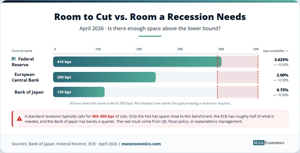
The first is the asymmetry of policy space. Central banks have demonstrated they can hike rates aggressively when inflation surges, as the Fed did from 0% to 5.5% in eighteen months between 2022 and 2024. That kind of move has plenty of room above the current rate. But the room below the current rate is narrow. If the Fed funds rate is 3.625% and the neutral rate is 3.0%, only about 60 basis points of conventional easing exists before policy is neutral, and another 300 basis points before it hits zero. A standard recession typically calls for 400–500 basis points of cuts. The arithmetic does not work without QE or fiscal support, which means every central bank now plans for the trap as a base case rather than a tail risk. The Federal Reserve Bank of New York’s December 2025 communication emphasised that the FOMC ended balance-sheet runoff in December and immediately initiated reserve management purchases, a signal that the institutional infrastructure for unconventional policy is now permanent, not emergency.
The second change is the legacy of QE itself. Japan’s central bank holds half the outstanding stock of government bonds. The Fed’s balance sheet, even after years of quantitative tightening, remains above $6 trillion. The ECB’s APP and PEPP portfolios are running off “at a measured and predictable pace,” but the absolute size remains historically extreme. These balance sheets create their own distortions, including the asset price inflation we cover in our analysis of asset price inflation, and they constrain the next round of unconventional easing. There is a credibility ceiling on how large a balance sheet can grow before markets begin to question fiscal dominance, and that ceiling tightens the closer current balance sheets sit to it.
The third change is the renewed relevance of fiscal policy. The COVID-era response was the largest peacetime fiscal expansion in modern history, and it produced inflation. That episode fed the modern monetary theory debate, covered in our piece on modern monetary theory, but it also rehabilitated the older Keynesian view that fiscal policy is the appropriate tool when monetary policy is at the ELB. The 2025–2026 debate inside the eurozone about the “supportive effects of past interest rate cuts” and the “gradual rollout of public spending on defence and infrastructure” is, in technical terms, a debate about the policy mix at the lower bound. Japan’s situation, where Prime Minister Sanae Takaichi’s expansionary fiscal stance has driven 40-year JGB yields above 4% for the first time since 2007, illustrates the constraint from the other direction: fiscal expansion at low policy rates can break the bond market before it raises growth.
The applications are concrete. In the United States, the Fed’s monetary policy transmission lags mean that any move toward neutral takes effect with a delay, which compounds the asymmetry: by the time policy bites, the next downturn may already require unconventional tools. In the United Kingdom, the Bank of England faces the same dilemma with even less fiscal headroom following the 2022 mini-budget episode. In Canada and Australia, central banks have explicitly written ELB protocols into their policy frameworks, including standing commitments to use QE if rates approach zero. The frameworks differ in detail, but the architecture is the same: every advanced-economy central bank now treats the trap as a recurring constraint rather than an aberration. Bernanke’s 2002 speech, “Deflation: Making Sure ‘It’ Doesn’t Happen Here,” delivered when the Fed funds rate was 1.75%, has become a planning document.
The post-COVID inflation surge was a temporary escape from the trap. Inflation rose, expected inflation rose, and the real interest rate fell sharply even as nominal rates lagged. That allowed the central banks of advanced economies to move conventional policy back into a meaningful range. But the structural drivers that produced the original trap, including aging populations, sluggish productivity growth, high private and public debt loads, and a global savings glut, have not gone away. The IMF’s 2024 World Economic Outlook chapter on natural rates concluded that medium-term \( r^* \) for advanced economies remains 1–2 percentage points below pre-2008 levels. If that estimate is right, every recession brings the trap back into play.
MASEconomics Explains
Four economic concepts behind liquidity trap economics
Conclusion
Liquidity trap economics has become a structural feature of advanced‑economy monetary policy. The Bank of Japan’s quarter‑century at or near zero, the Federal Reserve’s seven‑year stay between 2008 and 2015, the eurozone’s decade with negative deposit rates, and the renewed proximity of all three central banks to the lower bound after the post‑pandemic cycle demonstrate this persistence. The asymmetry between the room to hike and the room to cut, the dependence on credibility and expectations rather than mechanical rate movements, and the renewed importance of fiscal coordination define the operating environment for every central bank in 2026.
Did you find this article helpful? Share it with someone who loves economics. And remember, at MASEconomics, we make complex ideas simple.