A Practical Guide to Causal Inference in Economics

Does raising the minimum wage destroy jobs? Does an extra year of education increase lifetime earnings? Did Germany’s reunification hurt its economy? These are among the most important questions in economics, and for most of the discipline’s history, they were nearly impossible to answer rigorously. The problem is deceptively simple: to know the effect of a policy, you need to know what would have happened without it. But you can never observe a world where the policy both did and did not happen at the same time.

This is the fundamental problem of causal inference, and solving it has been the defining intellectual challenge of modern empirical economics.

In 2021, the Nobel Prize in Economics was awarded to David Card, Joshua Angrist, and Guido Imbens for their contributions to this challenge. Their work, alongside that of Alberto Abadie, Matias Cattaneo, and others, has produced a toolkit of quasi-experimental methods that allow economists to estimate causal effects from observational data with a credibility that approaches that of randomized controlled trials. This transformation has been called the “credibility revolution,” and it has reshaped how empirical research is conducted across every subfield of economics.

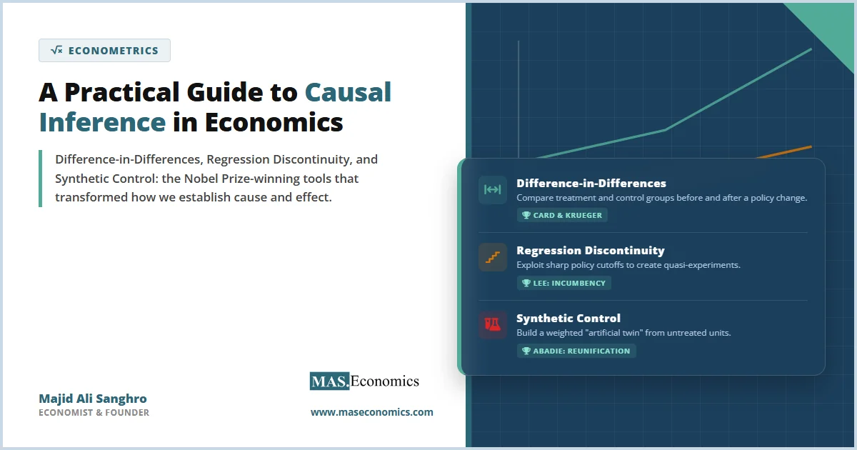
A practical guide to three key econometric methods: Difference-in-Differences (DiD), Regression Discontinuity Design (RDD), and the Synthetic Control Method (SCM).

Correlation Is Not Causation

Every introductory research methods course teaches that correlation does not imply causation. But appreciating why this matters requires understanding the concept of the counterfactual.

Suppose a government introduces a job training program for unemployed workers. Six months later, participants have higher employment rates than non-participants. Can we conclude that the program caused the improvement? Not necessarily. The participants may have been more motivated to find work than non-participants, meaning they would have found jobs anyway. Or the economy may have improved during the six months, lifting employment for everyone. The observed difference in outcomes between participants and non-participants mixes the genuine effect of the program with these other factors, which economists call confounders.

The gold standard for eliminating confounders is a randomized controlled trial (RCT), where individuals are randomly assigned to treatment and control groups. Randomization ensures that, on average, the two groups are identical in every respect except the treatment, so any difference in outcomes must be caused by the treatment itself. But in economics, RCTs are often impractical or unethical. We cannot randomly assign countries to different fiscal policies, randomly assign workers to different minimum wages, or randomly reunify half of Germany.

This is where quasi-experimental methods come in. They exploit features of the real world, such as policy changes, eligibility thresholds, and geographic variation, that create something resembling a natural experiment. The genius of these methods is that they use the structure of the policy itself to construct the counterfactual that an RCT would have provided.

Method 1: Difference-in-Differences (DiD)

Difference-in-Differences is the workhorse of modern policy evaluation. The method compares the change in outcomes over time between a group that is affected by a policy (the treatment group) and a group that is not (the control group). By taking the difference in the differences, the method removes both time-invariant characteristics of each group and common time trends that affect both groups equally.

The logic is elegant. Suppose you want to estimate the effect of a new minimum wage law in one state. You observe employment in that state before and after the law, and you also observe employment in a neighboring state that did not change its minimum wage. The change in employment in the neighboring state captures what would have happened in the treated state in the absence of the policy (the counterfactual). The difference between the actual change in the treated state and the counterfactual change in the control state is the estimated causal effect of the minimum wage.

Mathematically, the DiD estimator is:

τ_DiD = (Y̅_{treated, after} − Y̅_{treated, before}) − (Y̅_{control, after} − Y̅_{control, before})

The Landmark Application: Card and Krueger’s Minimum Wage Study

The most famous DiD study in economics is Card and Krueger (1994), which examined the effect of New Jersey’s minimum wage increase from $4.25 to $5.05 per hour in April 1992. Using fast-food restaurants in eastern Pennsylvania, where the minimum wage did not change, as the control group, Card and Krueger found that employment actually increased in New Jersey relative to Pennsylvania after the wage hike. This finding challenged decades of economic orthodoxy that predicted minimum wage increases would reduce employment, and it fundamentally changed the policy debate around minimum wages worldwide.

The Key Assumption

DiD only produces valid causal estimates if the treatment and control groups would have followed the same trend in the absence of the treatment. This is the parallel trends assumption. In the Card and Krueger example, it means that fast-food employment in New Jersey and Pennsylvania would have changed by the same amount if New Jersey had not raised its minimum wage.

This assumption cannot be directly tested because we never observe the counterfactual. However, researchers can provide supporting evidence by showing that the two groups followed parallel trends in the pre-treatment period. If employment in New Jersey and Pennsylvania was moving in lockstep before the policy change, it is more plausible that they would have continued to do so afterward.

The New DiD Revolution

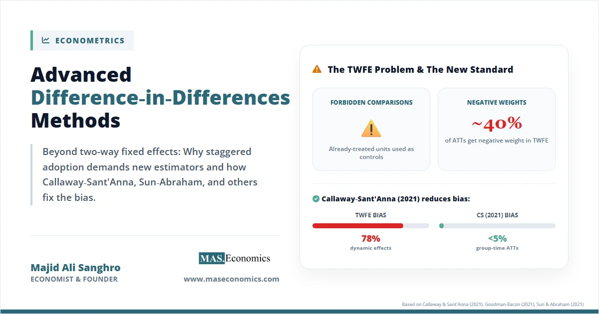
Since 2020, a wave of methodological innovation has transformed how DiD is implemented. Researchers, including Callaway and Sant’Anna, Borusyak, Jaravel, Spiess, and de Chaisemartin and D’Haultfoeuille, have shown that the traditional two-way fixed effects (TWFE) estimator, the most commonly used DiD implementation, can produce severely biased estimates when treatment is staggered across time, meaning different units receive treatment at different times.

The problem is that TWFE uses already-treated units as part of the control group for later-treated units, which contaminates the estimates. The new “heterogeneity-robust” DiD estimators address this by carefully defining which comparisons are valid. These advances have led to widespread reanalysis of existing studies, and in some cases, the results have changed substantially. Any researcher conducting a DiD study in 2026 should be using these newer methods rather than the traditional TWFE approach.

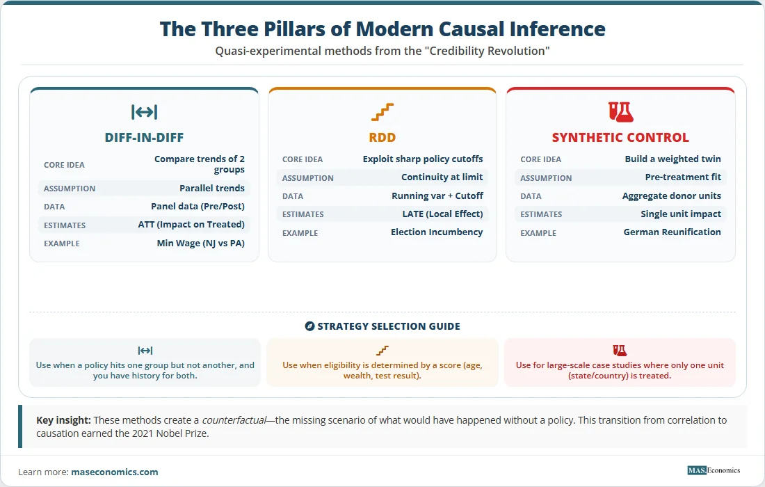
Feature	Difference-in-Differences	Regression Discontinuity	Synthetic Control
Core idea	Compare treated vs control, before vs after	Compare units just above and below a policy cutoff	Build a weighted artificial counterfactual
Key assumption	Parallel trends in absence of treatment	Continuity of potential outcomes at cutoff	Good pre-treatment fit from donor pool
Type of effect estimated	Average Treatment Effect on the Treated (ATT)	Local Average Treatment Effect (LATE) at cutoff	Treatment effect on the specific treated unit
Data requirements	Panel data with pre/post observations	Running variable with known cutoff	Aggregate panel data with donor units
Typical application	Policy rollouts, law changes, program introductions	Age/income thresholds, exam scores, election margins	Country/state-level policy changes with few treated units
Credibility ranking	High (with parallel trends evidence)	Very high (near-experimental at cutoff)	High (with transparent weighting)

Method 2: Regression Discontinuity Design (RDD)

Regression Discontinuity exploits situations where treatment is assigned based on whether a continuous variable, called the running variable, crosses a specific threshold. Because individuals just above and just below the threshold are nearly identical in all respects except their treatment status, comparing their outcomes provides a highly credible estimate of the causal effect of the treatment.

The intuition is beautiful in its simplicity. Consider a scholarship program that awards funding to students who score above 80 on an exam. A student who scored 81 receives the scholarship; a student who scored 79 does not. Are these two students fundamentally different? With hundreds of students near the cutoff, the answer is no, they are essentially the same population separated by a few points of luck or measurement noise. Any difference in their subsequent outcomes, such as college completion or earnings, can be attributed to the scholarship.

As Charles Darwin wrote, “Nature does not make jumps.” In the context of RDD, this means that if we observe a sudden jump in outcomes right at the threshold, we can be confident that the jump is caused by the treatment, because everything else changes smoothly and continuously across the cutoff.

Lee’s Incumbency Advantage Study

One of the most influential RDD applications is David Lee’s study of incumbency advantage in US House elections. In a two-party election, the winning candidate is the one who gets just over 50% of the vote. Lee compared the subsequent electoral performance of candidates who barely won their first election (51% of the vote) with those who barely lost (49%). Because these candidates are essentially identical except for the narrow margin of victory, any difference in their future success can be attributed to the causal effect of incumbency. Lee found that winning by a narrow margin increased the probability of winning the next election by 40 to 45 percentage points, a massive incumbency advantage.

The Key Assumption

RDD requires that, in the absence of treatment, the expected outcome would change smoothly across the cutoff. If something else also changes at the cutoff, the design is invalid. For example, if students who scored above 80 also received extra tutoring from a separate program, the jump in outcomes at 80 could be due to the tutoring rather than the scholarship.

A critical threat to RDD is the manipulation of the running variable. If students can precisely control their exam scores to land just above the threshold, the units above and below the cutoff are no longer comparable. Researchers routinely test for this by examining whether the density of the running variable shows a suspicious bunching at the cutoff, using what is known as a McCrary density test.

Sharp vs. Fuzzy RDD

In a sharp RDD, treatment is perfectly determined by the cutoff: everyone above receives treatment, everyone below does not. In a fuzzy RDD, the cutoff changes the probability of treatment but does not determine it perfectly. For instance, students above the cutoff may be eligible for a scholarship but not all of them accept it, and some below the cutoff may receive it through appeals. Fuzzy RDD uses the cutoff as an instrumental variable and estimates a Local Average Treatment Effect (LATE) for those whose treatment status is actually changed by the cutoff.

Method 3: Synthetic Control Method (SCM)

The Synthetic Control Method addresses a situation that DiD and RDD cannot easily handle: what happens when only one unit, or very few units, receive treatment? If California passes a unique policy and you want to estimate its effect, you cannot simply compare California to another state, because no single state is a perfect control. Synthetic Control solves this by constructing a weighted combination of multiple untreated states that, together, closely match California’s pre-treatment characteristics and outcomes.

The resulting “synthetic California” is a data-driven counterfactual that represents what would have happened to California without the policy. The treatment effect is estimated as the gap between California’s actual outcome and the synthetic California’s predicted outcome after the policy takes effect.

Abadie and Gardeazabal’s Study of German Reunification

Alberto Abadie, Alexis Diamond, and Jens Hainmueller’s study of German reunification is the foundational application of the Synthetic Control Method. The question was: what was the economic cost of reunification for West Germany? Since no other country experienced an equivalent shock, there was no natural control group. The researchers constructed a “synthetic West Germany” from a weighted combination of Austria, the United States, Japan, the Netherlands, and Switzerland. This synthetic version closely matched West Germany’s GDP per capita trajectory before reunification but diverged sharply afterward, revealing a significant negative effect of reunification on West Germany’s GDP per capita.

The Key Assumption

Synthetic Control is credible when the synthetic unit closely matches the treated unit’s outcomes during the pre-treatment period. If the match is poor, the post-treatment gap cannot be reliably attributed to the treatment. The method also requires that the donor pool, the set of potential control units, is large enough and diverse enough to construct a good match. Transparency is a key advantage: researchers can show exactly which units received what weight and how well the synthetic unit tracks the treated unit before treatment.

Inference and Robustness

Because SCM typically involves a single treated unit, traditional statistical inference based on large-sample theory does not apply. Instead, researchers use permutation tests (also called placebo tests): they apply the synthetic control method to each untreated unit in the donor pool, pretending each one was treated. If the estimated effect for the truly treated unit is much larger than the placebo effect, the result is considered statistically significant. This is an intuitive and transparent approach to inference that does not rely on distributional assumptions.

The chart illustrates the explosive growth of causal inference methods in the economics literature. Difference-in-Differences, already established by the early 1990s, has grown roughly 160-fold. Regression Discontinuity barely existed before 1999, but has become one of the most widely used methods. Synthetic Control, the newest of the three, has grown from a single paper in 2003 to hundreds of annual applications. Together, these three methods now account for a substantial share of all empirical economics research published in top journals.

How to Choose the Right Method

Choosing between these methods depends on the structure of the research question and the available data. Here is a practical decision framework.

Use Difference-in-Differences when: A policy or program affects some units (states, firms, individuals) but not others, and you have data from before and after the policy. You need a plausible control group that was following a similar trend before the policy change. DiD is ideal for studying the effects of new laws, trade policies, tax changes, and program rollouts.

Use Regression Discontinuity when: Treatment is assigned based on a continuous variable crossing a threshold, such as an age cutoff, an income threshold, an exam score, or an election margin. You need enough observations near the cutoff to make meaningful comparisons. RDD is ideal for studying the effects of eligibility rules, licensing requirements, and age-based policies.

Use Synthetic Control when: Only one or a few units receive treatment, such as a single country adopting a new policy, a single state implementing a unique reform, or a single city hosting a major event. You need a donor pool of similar untreated units and sufficient pre-treatment data to construct a credible synthetic counterfactual. SCM is ideal for studying country-level policy changes, state-level reforms, and unique historical events.

The Credibility Revolution and Its Impact

The rise of these methods has transformed economics from a discipline often criticized for relying on unreliable correlations to one that produces some of the most credible causal evidence in the social sciences. As the Royal Swedish Academy noted when awarding the 2021 Nobel Prize, the work of Card, Angrist, and Imbens “has substantially improved our ability to answer key causal questions” and “revolutionized empirical research” across the social sciences.

The practical consequences are enormous. These methods have provided rigorous evidence on questions that matter directly to people’s lives: the effect of minimum wages on employment, the returns to education, the impact of immigration on native workers, the effectiveness of job training programs, the costs of environmental regulations, and hundreds of other policy questions. Governments around the world now use these methods routinely in policy evaluation, and no serious empirical economics paper can be published in a top journal without addressing causal identification.

Mastering these methods is no longer optional. Today, around 50% of empirical economics articles focus on causal inference, and this share is even higher in applied fields like labour, development, health, and education economics. Understanding DiD, RDD, and SCM is essential for anyone who wants to contribute to or critically evaluate modern economic research.

MASEconomics Explains

Key Takeaway and Conclusion

Causal inference is the art and science of answering the most important question in economics: Does X actually cause Y? The three methods covered in this guide, Difference-in-Differences, Regression Discontinuity, and Synthetic Control, represent the most powerful tools economists have developed for answering that question using real-world data.

Each method exploits a different feature of the research setting to construct a credible counterfactual. DiD uses the time path of a control group. RDD uses a sharp threshold that creates a near-experiment. SCM uses a weighted combination of untreated units to build an artificial twin. Together, they form the core of the credibility revolution that has transformed economics from a field of disputed correlations into one that produces actionable, policy-relevant causal evidence.

For aspiring economists and data scientists, these are not just academic techniques. They are practical tools that governments, international organizations, and businesses use every day to evaluate policies, design interventions, and make decisions. Mastering them opens the door to rigorous empirical research on the questions that matter most to society.

The 2021 Nobel Prize recognized that these methods have “substantially improved our ability to answer key causal questions.” But the real significance is simpler: they allow us to move beyond “we think this policy works” to “we have credible evidence that this policy works.” In a world drowning in data but starving for reliable evidence, that distinction has never been more important.

Did you find this article helpful? Share it with someone who loves economics. And remember, at MASEconomics, we make complex ideas simple.