In 1991, Joshua Angrist and Alan Krueger published a now-famous study that used a person’s quarter of birth as an instrument for years of schooling, exploiting the fact that compulsory-schooling laws interact with school-entry cutoffs to push slightly more education onto people born early in the year. The design was clever, and the dataset was enormous, more than 300,000 men from the US Census. Four years later, John Bound, David Jaeger, and Regina Baker showed that the link between quarter of birth and schooling was so faint that the instruments behaved almost like random noise, and that adding more of them made the estimates drift toward the very bias the method was supposed to remove. That episode is the textbook case of weak instruments: instruments that satisfy the logic of the method on paper but are too weakly correlated with the variable being instrumented to deliver trustworthy estimates in practice.
Instrumental variables estimation is built to handle endogeneity, the situation where a regressor is correlated with the error term and ordinary least squares is therefore biased. The method works by isolating the part of the problematic regressor that is driven by an outside instrument, then using only that clean variation to estimate the effect of interest. The entire argument rests on one quantity: how strongly the instrument moves the endogenous regressor. When that relationship is strong, IV recovers a consistent estimate. When it is weak, the estimator’s good properties collapse, often quietly, and the usual standard errors and confidence intervals stop meaning what they appear to mean.
What an Instrument Is Supposed to Do
Consider a simple model with one endogenous regressor. The outcome equation is the relationship we care about, and the first stage is the relationship between the instrument and the endogenous regressor.
Structural and First-Stage Equations
The parameter \(\pi\) is the heart of the matter. It measures instrument relevance, the degree to which the instrument actually shifts the endogenous regressor. The two-stage least squares (2SLS) estimator can be written as a ratio that makes the role of \(\pi\) explicit.
2SLS Estimator, Single Instrument
Read that second fraction carefully, because it explains the whole problem. The numerator is the sample covariance between the instrument and the structural error. In a valid design this is zero in expectation, but in any finite sample it is a small random number rather than exactly zero. The denominator is the sample covariance between the instrument and the endogenous regressor, which is governed by \(\pi\). When \(\pi\) is large, the denominator is large, the small random numerator gets divided down to almost nothing, and the estimator sits close to the true \(\beta\). When \(\pi\) is near zero, the denominator is tiny, and dividing a small random number by another small number produces an estimate that swings wildly. A weak instrument is precisely a small denominator, and a small denominator magnifies whatever noise sits in the numerator.
This is why the foundational logic of instrumental variables estimation can hold perfectly while the estimate is still useless. Exogeneity and relevance are separate conditions. An instrument can be flawlessly exogenous and still be so weakly relevant that the method fails to deliver.
How Weakness Biases the Estimator Toward OLS
The deeper damage is that weak instruments do not just add noise, they add bias, and the bias points in a predictable direction. The reason traces back to the first stage. In 2SLS, the endogenous regressor is replaced by its fitted value from the first-stage regression on the instruments. When instruments are strong, those fitted values capture genuine exogenous variation. When instruments are weak, the first-stage regression is mostly fitting sampling noise, and that fitted noise is correlated with the same structural error that contaminated OLS in the first place.
The result is that the 2SLS estimator becomes biased in the same direction as ordinary least squares. As relevance falls to zero, 2SLS does not converge on an unbiased answer, it collapses back toward the OLS estimate it was meant to correct. The expected bias of 2SLS relative to the bias of OLS is approximately governed by the strength of the first stage.
Approximate Relative Bias
This expression makes the famous diagnostic threshold intuitive. If the expected first-stage F is around 10, the relative bias is roughly one-ninth, or about 11 percent of the OLS bias. Push the F down to 2, and the relative bias is nearly 100 percent. The estimator has not failed loudly; it has silently slid back to the answer it was supposed to improve on, while still wearing the appearance of a corrected estimate.
Warning. Weak instruments produce bias toward OLS, not toward zero. An IV result that looks suspiciously close to the OLS result it was meant to fix may not be reassuring agreement between methods. It may be the signature of a weak first stage dragging the IV estimate back toward the biased OLS answer.
A Worked Example: Watching the Denominator Shrink
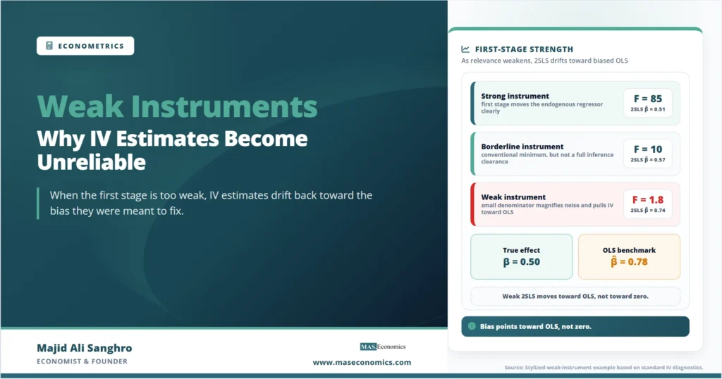
Consider a stylized example with internally consistent numbers. Suppose the true effect is \(\beta = 0.5\), the endogenous regressor is positively correlated with the error so OLS is biased upward, and an analyst has one candidate instrument. The table below shows what happens to the same estimator across three first-stage strengths, holding everything else fixed. The instrument-error covariance in the numerator is the same small sampling artifact in every column; only the first-stage strength changes.
| First-stage strength | First-stage \(\hat{\pi}\) | First-stage F | 2SLS estimate of \(\beta\) | Effective reliability |
|---|---|---|---|---|
| Strong instrument | 0.60 | 85.0 | 0.51 | Close to true \(\beta = 0.5\) |
| Borderline instrument | 0.18 | 10.2 | 0.57 | Noticeable bias toward OLS |
| Weak instrument | 0.05 | 1.8 | 0.74 | Severe bias, unstable across samples |
| OLS benchmark | — | — | 0.78 | Biased target the weak case drifts toward |
|
Source: Stylized example based on standard formulas. Numbers chosen for illustration.

|
||||
The pattern is the point. In the strong case the IV estimate sits near the truth and well away from the biased OLS benchmark of 0.78. As the first stage weakens, the IV estimate marches steadily toward that benchmark. By the time the F-statistic falls below 2, the IV estimate of 0.74 is barely distinguishable from the OLS estimate it was supposed to repair. The method has not announced its failure. The coefficient still has a standard error, the regression still runs, and a reader who does not inspect the first stage would have no signal that anything is wrong.
The First-Stage F-Statistic and the Rule of Ten
The practical diagnostic that emerged from this literature is the first-stage F-statistic, which tests the joint hypothesis that the instruments have no explanatory power for the endogenous regressor. In the seminal treatment, Staiger and Stock (1997) developed the asymptotic theory for IV under weak instruments and proposed the rule of thumb that, with a single endogenous regressor, instruments should be treated as weak if the first-stage F is below 10. Stock and Yogo (2005) later put this on firmer footing by deriving critical values tied to explicit tolerances, such as how much relative bias or size distortion a researcher is willing to accept.
The logic behind the number 10 follows directly from the relative-bias expression above. An expected first-stage F of about 10 corresponds to roughly 10 percent maximum bias of 2SLS relative to OLS, which the original authors judged to be a defensible ceiling for applied work. The threshold was never meant to be a law of nature. It was a convenient summary of a continuous relationship between first-stage strength and estimator reliability.
| First-stage F | Approx. relative bias | Interpretation | Recommended response |
|---|---|---|---|
| Below 5 | Above 25% | Instruments are weak | Do not rely on standard 2SLS inference |
| Around 10 | About 10% | Conventional minimum for relevance | Treat as a floor, not a clearance |
| 10 to 100 | Below 10% | Strong by the classic rule, but t-test size may still be distorted | Consider weak-instrument-robust inference |
| Above 104.7 | Negligible | Strong enough for valid conventional t-ratio inference | Standard 2SLS inference is reliable |
|
Source: Thresholds from Staiger and Stock (1997), Stock and Yogo (2005), and Lee, McCrary, Moreira, and Porter (2022).
|
|||
The final row deserves attention because it reflects a substantial revision to standard practice. In Valid t-Ratio Inference for IV, Lee, McCrary, Moreira, and Porter (2022) showed that the familiar rule of ten is far too lax if the goal is a trustworthy t-test rather than merely limited bias. They demonstrated that a true 5 percent test using the conventional critical value of 1.96 requires a first-stage F above roughly 104.7, and that keeping 10 as the threshold would require inflating the critical value to about 3.43. Reexamining 61 published papers in the American Economic Review, they found that correcting inference this way turned a large share of headline-significant results insignificant. The takeaway is not that the rule of ten was foolish, but that clearing it guarantees only modest bias, not the reliable confidence intervals that applied work routinely assumes.
Why More Instruments Makes the Problem Worse, Not Better
A natural instinct, when a single instrument is weak, is to add more instruments in the hope that several mediocre ones combine into something strong. This usually backfires. Each additional instrument that contributes little genuine first-stage explanatory power adds to the overfitting of the first stage. The fitted values absorb more sampling noise, that noise correlates with the structural error, and the bias toward OLS intensifies. This is exactly the mechanism Bound, Jaeger, and Baker identified in the quarter-of-birth study: the specifications with the largest number of instruments, including interactions, were the ones whose estimates drifted closest to the biased OLS result, even though the larger instrument set raised the apparent precision.
The same caution applies in the generalized method of moments framework, where overidentification with many moment conditions can deliver impressively tight standard errors while the underlying identification is thin. Precision that comes from weak, numerous instruments is precision around the wrong number. The diagnostic question is never how many instruments there are, but how much real first-stage variation they collectively explain.
Caveat. The first-stage F is itself estimated, and pre-testing on it introduces its own distortions. Selecting a specification because its F cleared 10 changes the sampling distribution of the estimate that follows. The cleaner approach is to report the first stage transparently and, when relevance is in doubt, use inference methods that remain valid regardless of instrument strength.
What to Do When Instruments Are Weak
The most important response is diagnostic honesty. The first stage should always be reported, including the F-statistic and the coefficients on the instruments, so that readers can judge relevance for themselves. Staiger and Stock noted that in their review of applied work, first-stage statistics were frequently absent from published tables, which left readers unable to assess whether the IV machinery was doing anything at all. Reporting the first stage is the single cheapest safeguard against the weak-instrument trap.
When relevance is genuinely in doubt, the better path is weak-instrument-robust inference, which constructs confidence sets that have correct coverage even when the first stage is weak. The classic tool is the Anderson-Rubin test, introduced in 1949 and revived as a workhorse precisely because its size does not depend on instrument strength. The tF procedure of Lee and coauthors offers a related correction, scaling the t-ratio critical value smoothly with the observed first-stage F. Limited information maximum likelihood, or LIML, is another estimator that is less biased than 2SLS under weak identification, though it is not immune. The common thread is that these methods stop pretending the first stage is strong and instead build the uncertainty about relevance directly into the inference.
Some problems, though, cannot be patched at the estimation stage. If an instrument is fundamentally weak because the underlying natural experiment barely moves the regressor, no robust test can manufacture identifying power that the data do not contain. In that situation the honest conclusion is that the design does not identify the effect with useful precision, and the search must turn to a stronger source of exogenous variation. A well-chosen natural experiment that shifts the endogenous regressor sharply is worth more than a dozen clever but feeble instruments.
Where Weak Instruments Sit in the Wider Toolkit
Weak instruments are one member of a family of identification problems that share a common shape: an estimator that is consistent in theory becomes unreliable in finite samples because some key quantity is too small to do its job. The endogeneity that motivates IV in the first place is the reason ordinary regression fails, and the foundations of that problem are covered in the treatments of simple linear regression and multiple regression models. The weak-instrument diagnostic is, in a sense, a relevance check layered on top of those foundations.
The likelihood-based alternative, LIML, connects to the broader logic of maximum likelihood estimation, where the estimator is chosen to best explain the observed data rather than to satisfy a moment condition mechanically. And the danger that weak first stages pose to inference parallels the selection problems addressed by the Heckman selection model, where ignoring a hidden correlation quietly contaminates an otherwise clean estimate. Seen this way, the lesson of weak instruments is not narrow. It is a reminder that consistency is an asymptotic promise, and that the finite-sample reality depends on whether the data actually contain the variation a method assumes.
Explains
Three ideas that make the weak-instrument problem click
Build your econometrics foundations one diagnostic at a time.
Explore the MASEconomics BlogConclusion
The problem of weak instruments is fundamentally a problem of a vanishing denominator. The two-stage least squares estimator divides a small, noisy instrument-error covariance by the instrument-regressor covariance, and when that second quantity is near zero, the estimator inherits all the instability and bias of dividing one small number by another. Far from converging on an unbiased answer, a weakly identified IV estimate drifts back toward the biased OLS result it was designed to correct, and it does so without any visible alarm in the output.
The first-stage F-statistic is the central diagnostic, and the rule that it should exceed 10 captures the point at which relative bias falls to roughly 10 percent. More recent work has shown that reliable t-ratio inference demands a far higher bar, near 104.7, which reframes the classic threshold as a floor for bias rather than a clearance for inference. Adding instruments does not rescue a weak design and often worsens it, because numerous feeble instruments overfit the first stage and tighten standard errors around the wrong estimate. The durable response is to report the first stage openly, to use weak-instrument-robust methods when relevance is uncertain, and to recognize when a design simply lacks the identifying power to answer the question. Instrumental variables remain one of the most powerful ideas in applied econometrics, but its power is borrowed entirely from the strength of the instrument, and a weak instrument has nothing to lend.
Frequently Asked Questions
What is the rule of thumb for weak instruments?
The traditional rule, from Staiger and Stock (1997), treats instruments as weak when the first-stage F-statistic is below 10, which corresponds to roughly 10 percent bias of 2SLS relative to OLS. Lee, McCrary, Moreira, and Porter (2022) showed that reliable t-ratio inference using the standard 1.96 critical value actually requires a first-stage F above about 104.7, so the rule of ten is best read as a minimum for limiting bias rather than a guarantee of trustworthy confidence intervals.
Why do weak instruments bias estimates toward OLS?
In 2SLS the endogenous regressor is replaced by its fitted value from the first stage. When instruments are weak, that fitted value is mostly sampling noise, and the noise is correlated with the same structural error that biased OLS. As a result the IV estimate inherits the OLS bias, and as instrument strength falls to zero the IV estimate collapses toward the OLS answer it was meant to correct.
Does adding more instruments fix weak identification?
Usually not. Adding instruments that contribute little genuine first-stage explanatory power increases overfitting of the first stage, which intensifies the bias toward OLS while making standard errors look deceptively small. The famous quarter-of-birth study is the cautionary case: specifications with the most instruments produced estimates closest to the biased OLS result. Strength comes from how much real variation the instruments explain, not from their number.
What can you do when instruments are weak?
Always report the first stage, including the F-statistic and instrument coefficients. When relevance is in doubt, use weak-instrument-robust inference such as the Anderson-Rubin test or the tF procedure, which give confidence sets with correct coverage regardless of instrument strength. LIML is also less biased than 2SLS under weak identification. If the instrument fundamentally fails to move the regressor, no correction can manufacture identifying power, and a stronger source of exogenous variation is needed.
How is instrument relevance different from instrument exogeneity?
Exogeneity means the instrument is uncorrelated with the structural error, so it does not affect the outcome except through the endogenous regressor. Relevance means the instrument is correlated with the endogenous regressor in the first place. Both are required for valid IV. The weak-instrument problem is a failure of relevance, not exogeneity: the instrument may be entirely clean yet still too weakly linked to the regressor to produce a reliable estimate.
Thanks for reading! If you found this helpful, share it with friends and spread the knowledge. Happy learning with MASEconomics