Causal Machine Learning for Economists: Double ML and Causal Forests Explained

For decades, applied econometrics has lived with an uncomfortable trade-off. To get unbiased causal estimates, researchers leaned on linear regression, instrumental variables, and propensity score methods. These tools work well when the number of controls is small and the relationships are roughly linear. They struggle when the world is high-dimensional, non-linear, and full of treatment effects that vary across people, places, and time. Causal machine learning was built to close that gap. It borrows the predictive flexibility of modern machine learning, then disciplines those predictions using the identification logic of econometrics. The result is a family of estimators that can handle hundreds of controls, recover unbiased average effects, and reveal how those effects differ across the population.

This article explains the two methods that have done the most to push causal machine learning into mainstream economics: Double/Debiased Machine Learning (Double ML) developed by Chernozhukov and co-authors in 2018, and Causal Forests, formalised by Athey, Tibshirani, and Wager in 2019. Both methods now sit inside open-source libraries that thousands of researchers use every week, and both have changed how economists think about high-dimensional confounding and effect heterogeneity. The aim here is to give a working understanding of the mechanics, the assumptions, the empirical track record, and the policy use cases without losing the mathematical content that makes these methods rigorous.

What Causal ML Solved

Consider a familiar empirical question: Does eligibility for a 401(k) plan increase household savings? The challenge is selection. Workers at firms that offer 401(k) plans differ from workers at firms that do not in earnings, in education, in family structure, and in financial literacy. A naive comparison of savings between the two groups confuses the effect of the plan with the effect of being the kind of person who ends up at a plan-offering firm. The textbook fix is to control for observable differences. But how many controls? Income, age, education, marital status, family size, home ownership, IRA participation, defined benefit coverage, and so on. Once interactions and non-linear transformations are added, the control set explodes. Ordinary least squares (OLS) regression handles this badly. With many controls relative to the sample size, OLS overfits. With non-linear effects, a linear specification gives a biased estimate of the treatment effect even when unconfoundedness holds.

Machine learning solves the prediction problem. Random forests, gradient boosting, and neural networks can fit complicated, non-linear relationships in high dimensions without overfitting catastrophically. The trouble is that machine learning was not built to estimate causal parameters. Plug a random forest into a regression of outcome on treatment and controls, and the estimated treatment effect is sometimes severely biased. Chernozhukov and colleagues showed that the bias comes from two sources: regularisation bias, because the ML estimator shrinks coefficients to control variance, and overfitting bias, because the same data are used to fit the nuisance functions and to estimate the treatment effect. Both sources are fatal for inference. Confidence intervals built on naive plug-in ML estimators do not have the right coverage, so any policy recommendation drawn from them is on shaky ground.

Causal machine learning fixes both problems. Double ML combines a clever choice of estimating equation, the Neyman-orthogonal score with sample splitting (cross-fitting), which together neutralise the bias from using flexible ML in the first stage. Causal Forests take a different route: they extend the random forest algorithm to estimate, at each point in covariate space, a local treatment effect rather than a local prediction. Both methods scale to high-dimensional settings, both produce valid confidence intervals under stated assumptions, and both have implementations that economists can use without writing the algorithm from scratch. The conceptual leap is to treat machine learning as a tool for estimating nuisance functions, while reserving the causal logic, orthogonality, sample splitting, and honest estimation for the parameter that actually matters.

Mechanics of Double ML and Causal Forests

Causal machine learning rests on the same basic identification framework that powers most of modern causal inference in economics. The researcher has data on an outcome \( Y \), a treatment \( D \), and a set of pre-treatment covariates \( X \). The goal is to estimate the average treatment effect (ATE) and increasingly, the conditional average treatment effect (CATE) \( \tau(x) = E[Y(1) – Y(0) | X = x] \) under the assumption that all confounders are observed. The difference between traditional methods and causal ML lies entirely in how the relationship between \( Y \), \( D \), and \( X \) is modelled.

Double ML in three steps

Double ML in its simplest form targets the partially linear model \( Y = D\theta_0 + g_0(X) + U \), where \( \theta_0 \) is the causal parameter of interest and \( g_0(X) \) is an unknown function of the controls. The treatment itself follows \( D = m_0(X) + V \), where \( m_0(X) \) is the propensity score (or its continuous analogue, the conditional expectation of the treatment given controls). The two nuisance functions \( g_0 \) and \( m_0 \) can be arbitrarily complex.

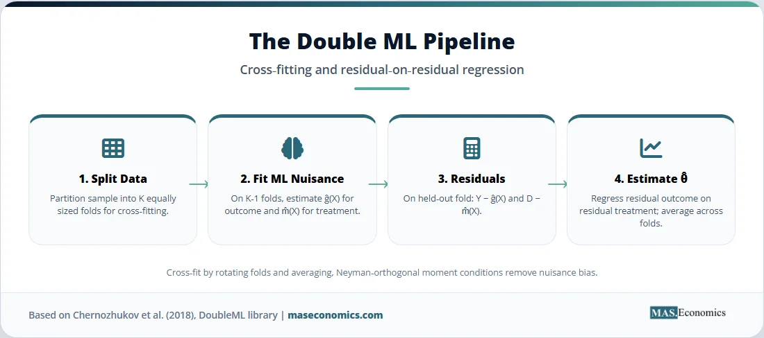
The estimation proceeds in three steps. First, split the sample into folds. Second, on each held-out fold, use a flexible ML method, such as random forests, gradient boosting, neural networks, lasso, or any combination, to estimate \( \hat{g}(X) \) and \( \hat{m}(X) \). Third, partial out the fitted nuisance functions and run a simple regression on the residuals: regress \( Y – \hat{g}(X) \) on \( D – \hat{m}(X) \). The coefficient from that residual-on-residual regression is the Double ML estimate of \( \theta_0 \). The procedure is then repeated by swapping fold roles and averaging the estimates, a step known as cross-fitting.

What makes this work is the combination of two ingredients. The first is Neyman orthogonality. The estimating equation for \( \theta_0 \) is constructed so that small errors in the nuisance estimates do not propagate into large errors in the parameter of interest. Formally, the derivative of the score with respect to the nuisance functions is zero at the truth. The second is sample splitting. By estimating the nuisance functions on one part of the data and using them to construct the score on a different part, the procedure removes the overfitting bias that would contaminate a single-sample plug-in estimator. Together, these two devices let \( \hat{\theta} \) achieve \( \sqrt{n} \)-consistency and asymptotic normality even when the underlying ML estimators converge at slower rates, as long as their convergence is at least \( n^{-1/4} \). The DoubleML package documentation provides a comprehensive practical reference to the implementation.

Causal Forests and honest splitting

Causal Forests pursue a different question. Rather than estimating one average effect, they estimate \( \tau(x) \) a separate treatment effect for every point in covariate space. The method extends Breiman’s random forest in two important ways.

First, the splitting rule changes. A standard regression tree splits to minimise prediction error in the outcome. A causal tree splits to maximise heterogeneity in the estimated treatment effect across child nodes. The split that creates the biggest difference in \( \hat{\tau} \) between the left and right children wins, subject to balance and overlap constraints. Across many trees, observations that the forest decides are similar in their treatment response will tend to land in the same leaves more often than observations whose responses differ. This adaptive weighting is the engine of CATE estimation.

Second, the trees are grown honestly. Each tree’s subsample is split into two parts: one is used to choose the splits, and the other is used to estimate the treatment effect inside each leaf. The two parts never overlap. Honest estimation eliminates the bias that would otherwise creep in from using the same observations to choose where to split and to compute the leaf-level effects. The cost is statistical efficiency; half the data are reserved for estimation rather than splitting, but the gain is valid asymptotic inference. Athey, Tibshirani, and Wager proved that, under regularity conditions, honest causal forests produce consistent and asymptotically Gaussian estimates of \( \tau(x) \), with confidence intervals that can be constructed from a forest-based variance estimator.

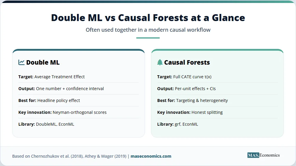
The two methods are complementary. Double ML targets a single causal parameter, typically the ATE, and gives the cleanest possible inference for that parameter. Causal Forests target the entire CATE function and reveal where the action is: which subgroups respond strongly to the policy, which do not respond at all, and which respond in the opposite direction. Many applied papers run both. Double ML provides the headline number; the forest provides the heterogeneity story behind it.

Causal ML in Equations

The mathematics of causal machine learning is dense in the original papers but pleasingly compact at the level of intuition. The key step in Double ML is the construction of the orthogonal score. Take the partially linear model:

A naive estimator of \( \theta_0 \) would regress \( Y \) on \( D \) after partialling out \( \hat{g}(X) \). The Neyman-orthogonal score uses both nuisance functions:

where \( W = (Y, D, X) \) and \( \eta = (g, m) \) is the nuisance pair. The orthogonality property is that \( \partial_\eta E[\psi(W; \theta_0, \eta)] = 0 \) at the true \( \eta_0 \). Small estimation errors in \( \hat{g} \) and \( \hat{m} \), therefore, enter the moment condition only through their product, a much weaker channel than additive contamination.

The Double ML estimator then solves the empirical analogue of \( E[\psi(W; \theta, \eta)] = 0 \) using cross-fitted estimates of \( \hat{g} \) and \( \hat{m} \). With \( K \)-fold cross-fitting, the estimator takes the form:

where \( \hat{g}^{(-k)} \) and \( \hat{m}^{(-k)} \) are estimated on the \( K – 1 \) folds excluding fold \( k \). Under regularity conditions including \( n^{-1/4} \) convergence of the ML nuisance estimators, the Double ML estimator satisfies \( \sqrt{n}(\hat{\theta}_{\text{DML}} – \theta_0) \xrightarrow{d} N(0, \sigma^2) \), with \( \sigma^2 \) consistently estimable from the cross-fitted residuals.

For Causal Forests, the building block is the local moment condition. The treatment effect \( \tau(x) \) at point \( x \) solves:

where \( \nu(x) \) collects local nuisance parameters such as the local intercept. In the simplest binary-treatment, unconfounded case, the score reduces to the Robinson-style residual product \( \psi_\tau(Y, D) = (Y – \mu(X))(D – e(X)) – \tau (D – e(X))^2 \), with \( \mu(X) = E[Y | X] \) and \( e(X) = E[D | X] \). The forest estimates \( \tau(x) \) by solving a weighted version of this equation:

where the weights \( \alpha_i(x) \) come from the forest itself: \( \alpha_i(x) \) is the fraction of trees in which observation \( i \) lands in the same leaf as the test point \( x \). Honest splitting and subsampling guarantee that \( \hat{\tau}(x) \) is asymptotically normal, with a variance estimator based on the bootstrap-of-little-bags procedure described in Athey, Tibshirani, and Wager.

Symbol	Meaning	Role in the model
\( Y \)	Outcome variable	What the analyst wants to explain
\( D \)	Treatment indicator or dose	The cause whose effect is being estimated
\( X \)	Covariate vector	Pre-treatment controls; can be high-dimensional
\( \theta_0 \)	Average treatment effect	Target parameter in Double ML
\( \tau(x) \)	Conditional average treatment effect	Target function in Causal Forests
\( g_0(X) \)	Outcome regression \( E[Y | X, D=0] \)	First nuisance function
\( m_0(X) \)	Propensity score \( E[D | X] \)	Second nuisance function
\( \psi(W; \theta, \eta) \)	Score function	Estimating equation; must be Neyman-orthogonal
\( \alpha_i(x) \)	Forest weight	Adaptive nearest-neighbour weight for observation \( i \) at point \( x \)
\( U, V \)	Idiosyncratic errors	Mean-zero residuals in outcome and treatment equations

The variable table summarises the moving parts. Notice how few symbols are needed once the abstraction is in place: an outcome, a treatment, a covariate vector, two nuisance functions, and a score. Everything else, the choice of ML method, the number of folds, and the splitting rule for the forest, is an implementation detail. That separation between identification and estimation is what makes causal machine learning portable across problems, from labour economics to digital marketing.

Assumptions of Causal ML

The validity of Double ML and Causal Forests rests on three core assumptions, all familiar from the program-evaluation literature. The first is unconfoundedness: conditional on \( X \), the treatment is independent of the potential outcomes. This is the same selection-on-observables assumption that powers regression adjustment, matching, and inverse probability weighting. Causal ML does not relax it. If an unobserved confounder drives both treatment and outcome, no ML method, however flexible, can recover the causal effect from observational data alone. Instrumental variable strategies remain the appropriate response when unconfoundedness fails.

The second is overlap, sometimes called common support: every unit must have a non-trivial probability of receiving each treatment level given its covariates, so \( 0 < m_0(X) < 1 \) holds for binary \( D \). When propensity scores approach zero or one in some regions of \( X \), the data contain little information about counterfactuals there, and any causal ML estimator included produces unstable or undefined effects. Trimming the sample to regions of adequate overlap is standard practice and recommended in the grf package documentation.

The third is high-quality nuisance estimation. Double ML’s \( \sqrt{n} \) inference theory requires the ML estimators of \( g_0 \) and \( m_0 \) to converge at a rate of at least \( n^{-1/4} \). For lasso, this translates into approximate sparsity. For random forests and gradient boosting, the rate depends on smoothness conditions on the underlying functions. In practice, researchers use cross-validation to tune the ML algorithms and check that residuals look reasonable, but the assumption is rarely tested directly. When it fails when the truth is too rough for the chosen ML method to learn fast enough, the asymptotic confidence intervals are not reliable.

Beyond these three core assumptions, several practical limitations deserve attention. Computational cost is real: a causal forest with 2,000 trees on a sample of 50,000 observations can take an hour to train on a standard laptop, and tuning across multiple candidate ML methods inside a Double ML pipeline multiplies that cost. Heterogeneity discovery is restricted to observable dimensions; if the true treatment effect varies along an unobserved characteristic, the forest cannot detect it. Causal forests can also produce noisy CATE estimates in regions of \( X \) with sparse data, and visual inspection of the heterogeneity plot is essential before drawing policy conclusions. Finally, when the instrument is weak or the identification is borderline, no amount of ML flexibility will rescue the analysis. Causal machine learning improves on traditional methods at the estimation stage; it does not change the identification logic.

Causal ML in Empirical Data

The empirical record for Double ML and Causal Forests is now substantial. The original Chernozhukov et al. (2018) paper revisits the question of whether 401(k) eligibility raises net financial assets, using a sample of around 9,900 households from the Survey of Income and Program Participation. With a rich set of controls, including income, age, family structure, IRA holdings, home ownership, defined benefit pension coverage, marital status, education, the authors compare Double ML estimates using lasso, random forests, gradient boosting, and neural networks against a naive plug-in ML estimator and a simple linear regression. The Double ML estimates cluster tightly across the different ML methods, with the average treatment effect on assets in the range of $9,000 to $11,000, depending on specification. The naive plug-in estimates, by contrast, are unstable and shifted, illustrating the bias that orthogonalisation and cross-fitting are designed to remove.

Simulation studies tell a similar story. When the data-generating process features non-linear confounding and a moderate-to-large number of controls, OLS shows large bias, propensity score matching shows substantial variance, and naive ML plug-in estimators show both. Double ML achieves bias close to zero and root mean squared error (RMSE) competitive with or better than the alternatives, with confidence intervals that achieve nominal coverage. The chart below summarises a representative pattern from the type of Monte Carlo experiments reported in the original paper and follow-up work, illustrating bias and RMSE for the four common approaches at sample size \( n = 2{,}000 \) with 50 confounders.

Source: Stylised illustration based on simulation patterns reported in Chernozhukov et al. (2018) and follow-up Monte Carlo studies. Values are illustrative magnitudes.

Causal Forests have an equally rich applied track record. Athey and Wager’s 2019 application paper applies the method to the National Study of Learning Mindsets, where a brief growth-mindset intervention was randomised across 76 schools. The forest reveals that students with low prior achievement gain the most, while students with high prior achievement gain little. That pattern would be invisible in a single ATE estimate. Other applied papers have used Causal Forests to study the heterogeneous effects of job training programs, microfinance access, advertising campaigns, electricity pricing, and tax credits. In each case, the headline ATE turns out to mask substantial variation across observable subgroups that has direct policy relevance.

The methods have also held up under stress tests. Bootstrap-based comparisons show that the asymptotic confidence intervals from Double ML achieve coverage close to the nominal level in moderate samples. Causal Forest confidence intervals are slightly undercovered when the CATE function is very wiggly, which is why analysts often supplement them with cross-validation diagnostics and out-of-bag predictions. The track record is not perfect, but it is good enough that both methods are now standard tools in applied work at central banks, tech firms, and economics departments.

Causal ML and Policy

The policy uses of causal machine learning fall into three categories, each of which is now visible in practice across the United States, the United Kingdom, Canada, and Australia. The first is a large-scale program evaluation with rich administrative data. Tax authorities, social security administrations, and education departments hold datasets with hundreds of variables on millions of individuals. Linear regression on such data either drops the bulk of the controls or imposes a restrictive functional form. Double ML lets analysts use everything in the data administrative records, geographic indicators, prior outcomes, and household composition without sacrificing inferential validity. The Internal Revenue Service in the US, His Majesty’s Revenue and Customs in the UK, and Statistics Canada have all released working papers using Double ML or closely related methods to study the effects of tax credits, audit policies, and benefit changes.

The second category is personalised policy. If a job training program raises earnings by an average of $1,500, but the effect ranges from $5,000 for displaced manufacturing workers to roughly zero for recent graduates, the policy implication is to target the program. Causal Forests deliver exactly the input that targeting requires: an estimate of \( \tau(x) \) for every individual, with a confidence interval. Adult education policy in Australia, active labour market policy in the United Kingdom, and health insurance design in the United States have all moved towards this targeting logic, and causal ML is the technical infrastructure behind much of it. The Australian Bureau of Statistics and the UK’s Behavioural Insights Team both publish methodological notes explaining how heterogeneous treatment effect estimation feeds into program design.

The third category is private-sector policy evaluation, particularly in technology platforms. Microsoft Research’s EconML library and Uber’s CausalML library exist because firms care about heterogeneous price sensitivities, customer-segment-specific advertising responses, and the marginal effect of platform features for different user groups. The same machinery that economists use to study labour market policy is used by data scientists to set prices and target promotions. The two-way flow of methods has accelerated development on both sides. Many of the recent improvements to Causal Forests, debiased estimation, instrumental variable extensions, and policy learning algorithms came out of industry research labs collaborating with academic econometricians.

Causal machine learning also fits naturally alongside the rest of the modern causal inference toolkit. Difference-in-differences with staggered adoption, regression discontinuity with high-dimensional running variables, and synthetic control methods have all been combined with Double ML to handle settings where the standard implementations break down. Machine learning more broadly is becoming embedded in econometric practice rather than sitting alongside it as a separate discipline. The same sample-splitting and orthogonalisation tricks that make Double ML work also underpin newer methods for quantile treatment effects, dynamic policy evaluation, and partial identification.

Looking forward, the frontier of causal machine learning is moving in three directions. The first is policy learning: methods that, instead of estimating treatment effects, directly recommend the optimal treatment assignment rule given a budget constraint. Athey and Wager’s policy learning framework, available in EconML and grf, takes this step. The second is sensitivity analysis for unconfoundedness: tools that quantify how much unobserved confounding would be needed to overturn a Double ML or Causal Forest result. The third is the integration of causal ML with structural economic models, so that flexible nuisance estimation feeds into welfare calculations and counterfactual policy simulations rather than stopping at the reduced-form effect. Each of these directions is being actively developed in working papers and open-source libraries, and economists who learn the basics of Double ML and Causal Forests today will be well placed to use them as the field continues to mature.

MASEconomics Explains

Conclusion

Causal machine learning has changed what applied econometrics looks like. Double ML solved the problem of unbiased estimation in high-dimensional settings by combining Neyman-orthogonal scores with cross-fitting. Causal Forests solved the problem of heterogeneous treatment effect estimation by extending random forests with honest splitting and adaptive weighting. Both methods come with rigorous asymptotic theory, both have open-source implementations in R and Python, and both have been validated in dozens of applied papers across labour economics, public finance, health, and industrial organisation. They do not replace careful research design; unconfoundedness, overlap, and quality controls remain non-negotiable, but they let economists exploit the full richness of modern administrative and platform data without sacrificing inferential validity. For any analyst working with high-dimensional controls or expecting effect heterogeneity, Double ML and Causal Forests are now the default tools, and learning them is no longer optional for serious causal work.

Did you find this article helpful? Share it with someone who loves economics. And remember, at MASEconomics, we make complex ideas simple.