In 1974, Clive Granger and Paul Newbold ran a simple Monte Carlo experiment that shook applied econometrics. They generated two completely independent random walks, regressed one on the other, and found “statistically significant” relationships in roughly three-quarters of their simulations. The variables had nothing to do with each other. The R-squared was high, the t-statistics looked respectable, and the entire result was a statistical illusion. Two decades of macroeconomic regressions, including many published in top journals, suddenly looked suspect.
The Augmented Dickey-Fuller test is the standard diagnostic that prevents this disaster. It tests whether a time series contains a unit root, which is the formal statistical condition that produces spurious regression. Real GDP, consumer price indices, exchange rates, and most macroeconomic aggregates almost always fail the test in levels and pass it in first differences. Knowing which case applies is the gate that determines whether ordinary least squares estimates can be trusted at all.
The test was developed by David Dickey and Wayne Fuller in 1979 and extended in 1981 to handle serial correlation in the residuals. Today, every central bank forecast, every IMF Article IV macroeconomic projection, and every academic time-series paper reports unit-root pre-testing as a baseline diagnostic. The procedure is short, the math is tractable, and the consequences of skipping it are severe.
The Spurious Regression Problem
Standard ordinary least squares assumes the variables in a regression have stable means, finite variances, and autocovariances that depend only on the lag between observations, not on calendar time. A series with these properties is called weakly stationary. Macroeconomic data almost never satisfy it. Real GDP grows. The price level rises. Exchange rates drift. The unconditional mean of the series moves with time, the variance can grow without bound, and the assumptions behind the t-statistic collapse.
The most common form of non-stationarity is the random walk, defined as \( y_t = y_{t-1} + \varepsilon_t \) where \( \varepsilon_t \) is white noise. The series has no mean-reverting force. A shock today persists forever in expectation. The variance grows linearly with time. Two independent random walks share no economic relationship, but because both wander upward over long horizons, a regression of one on the other will almost always produce a high R-squared and a large t-statistic. The standard distribution theory underlying inference no longer applies. This is what Granger and Newbold demonstrated, and the failure mode is called spurious regression.
The unit root is the precise mathematical condition. Consider the simple autoregressive process \( y_t = \rho y_{t-1} + \varepsilon_t \). When \( |\rho| < 1 \), the series is stationary, and shocks decay geometrically. When \( \rho = 1 \) the characteristic equation has a root on the unit circle, shocks are permanent, and the series is integrated of order one, denoted \( I(1) \). The Augmented Dickey-Fuller test is the formal hypothesis test for whether \( \rho = 1 \) against the stationary alternative \( \rho < 1 \).
Algebra of the ADF Test
Start with the autoregressive model of order one:
Subtract \( y_{t-1} \) from both sides. The transformation produces the workhorse equation of the entire unit-root literature:
The hypothesis on \( \rho \) translates directly into a hypothesis on \( \gamma \). The null of a unit root is now \( H_0: \gamma = 0 \) against the stationary alternative \( H_A: \gamma < 0 \). This is a one-sided test. A negative \( \gamma \) means \( \rho < 1 \) and shocks decay; a zero \( \gamma \) means \( \rho = 1 \) and shocks are permanent.
The simplest version, called the Dickey-Fuller test, regresses \( \Delta y_t \) on \( y_{t-1} \) and uses the t-statistic on \( \gamma \) as the test statistic. The catch is that under the null, this t-statistic does not follow a standard normal or Student’s t distribution. The denominator of the variance estimator is itself non-stationary under the null, and the asymptotic distribution of the statistic is non-standard. Dickey and Fuller derived the correct distribution and tabulated critical values via simulation.
The “augmented” version, introduced in 1981, addresses serial correlation in the residuals. Real economic series rarely follow a pure AR(1). Adding lagged differences of \( y_t \) as regressors absorbs the serial correlation and keeps the t-statistic on \( y_{t-1} \) asymptotically valid. The full ADF regression is:
Three specifications are nested inside this equation, each appropriate for a different class of series. The constant \( \alpha \) is omitted when the series has zero mean (rare with economic data). The trend term \( \beta t \) is included when the series has visible deterministic growth, such as real GDP or labour productivity. The pure random-walk specification drops both.
The test statistic is the t-ratio on \( \hat{\gamma} \):
The decision rule rejects the null when \( \tau \) is more negative than the critical value tabulated by MacKinnon (1996). At the 5% level, with a constant and no trend, the critical value is approximately \( -2.86 \). With a trend included it tightens to roughly \( -3.41 \). The standard normal critical value of \( -1.65 \) is far too lenient, which is why mechanical use of regression t-statistics under non-stationarity rejects the null too often and produces the spurious significance Granger and Newbold flagged.
Notation Reference
| Symbol | Definition |
|---|---|
| \( y_t \) | Observed time series at time \( t \) |
| \( \Delta y_t \) | First difference: \( y_t – y_{t-1} \) |
| \( \rho \) | Autoregressive coefficient on \( y_{t-1} \) |
| \( \gamma \) | Reparameterised coefficient: \( \rho – 1 \) |
| \( \alpha \) | Drift (constant) term |
| \( \beta t \) | Deterministic linear trend |
| \( p \) | Lag length on differenced regressors |
| \( \tau \) | ADF test statistic (t-ratio on \( \hat{\gamma} \)) |
| \( \varepsilon_t \) | White-noise innovation, mean zero |
 |
|
The ADF Testing Procedure
The mechanics of the test reduce to four computational steps, each of which has a defensible economic and statistical rationale.
The first step is choosing the deterministic specification. A visual inspection of the series usually settles the question. If the series shows clear secular growth, such as real GDP or UK real output, the trend term is included. If the series oscillates around a constant mean, such as the unemployment rate, the constant is included but the trend is dropped. Including unnecessary deterministic terms reduces the test’s power; omitting necessary ones biases the test toward failing to reject the null.
The second step is selecting the lag length \( p \). The augmented regression includes lagged differences specifically to soak up residual autocorrelation. Too few lags leave the residuals correlated and the test invalid. Too many lags consume degrees of freedom and reduce power. The standard data-driven rules use information criteria. The Akaike Information Criterion selects the \( p \) that minimises:
The Schwarz Bayesian Criterion penalises additional lags more heavily, replacing \( 2p \) with \( p \ln T \). Information-criterion model selection typically picks \( p \) between two and six for quarterly macroeconomic series. The Ng-Perron modified information criteria are now preferred in the academic literature because they correct a bias that conventional AIC and BIC display when the autoregressive root is close to one.
The third step is estimating the augmented regression by ordinary least squares and extracting the t-statistic on \( y_{t-1} \). The OLS estimator is consistent under the null, despite the non-stationarity of the regressor, because \( \Delta y_t \) is stationary on the left and the algebra of the t-ratio cancels the offending term. This is non-obvious and is why Dickey-Fuller had to derive a new distribution theory rather than borrow Wald’s standard results.
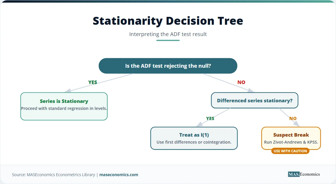
The fourth step is comparing the t-statistic to MacKinnon’s critical values. If \( \tau \) is more negative than the 5% critical value, the null of a unit root is rejected, and the series is treated as stationary. Otherwise, the null is not rejected, the series is treated as \( I(1) \), and the analysis proceeds in first differences. When the series is integrated of order one, the differenced series should pass the ADF test on its second application, confirming the order of integration.

Interpreting ADF Results: A UK GDP Example
Consider a stylized canonical example using UK real GDP from 1970 to 2020, fifty annual observations. The series displays the visible upward drift typical of long-run output data, with the global financial crisis of 2008-2009 and the COVID contraction of 2020 producing the only meaningful interruptions. The level series wanders upward; the first-differenced series, the annual growth rate, fluctuates around a mean of roughly two percent.
The ADF test is run twice: first on the level series with a constant and trend specification, then on the first-difference series with a constant only. Lag length is selected by the Schwarz criterion. The stylized canonical results are reported below.
| Series | Specification | ADF Statistic | 5% Critical Value | p-value | Decision |
|---|---|---|---|---|---|
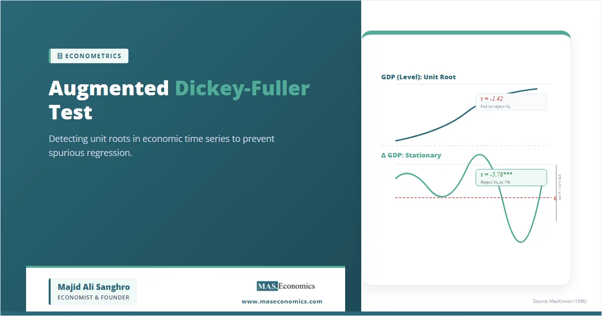
| Real GDP (level) | Constant + Trend | -1.42 | -3.41 | 0.572 | Fail to reject H0: Unit root present |
| Δ Real GDP (1st difference) | Constant only | -5.78*** | -2.86 | <0.001 | Reject H0: Stationary |
| Lag length (SBC) | 2 (level), 1 (first difference) | ||||
| Observations | 50 (level), 49 (first difference) | ||||
|
|||||
Note: *** p<0.01. Critical values from MacKinnon (1996). Stylized canonical example consistent with the literature on UK output stationarity.
Reading the output proceeds row by row. The level series produces a t-statistic of \( -1.42 \), well above the 5% critical value of \( -3.41 \). The associated p-value of 0.572 means there is no statistical basis for rejecting the unit root. UK real GDP behaves like a random walk with drift over this fifty-year window. Running an OLS regression of UK GDP on, say, US GDP, would produce the spurious-regression failure that motivated the entire test in the first place.
The first-differenced series is the annual growth rate. The ADF statistic on the differences is \( -5.78 \), far below the 5% critical value of \( -2.86 \) and significant at the 1% level. The null of a unit root is decisively rejected. UK GDP growth is a stationary series. The level is therefore integrated of order one, conventionally written \( y_t \sim I(1) \), and any subsequent regression analysis must either work in first differences or use cointegration techniques to recover long-run relationships.
Anatomy of an ADF output. The ADF statistic is the t-ratio on the lagged level term, more negative when the series mean-reverts strongly. The critical value is the percentile of the Dickey-Fuller distribution, which differs from a standard t. The p-value is the MacKinnon-derived probability of observing a statistic this extreme under the null. The decision follows the rule: reject the unit root only when the statistic is more negative than the critical value.
The chart below visualises the stationarity contrast that the ADF test formalises. The level series wanders without a stable mean. The first-differenced series oscillates within a narrow band around two percent and reverts to that mean after every shock. The visual difference matches the statistical verdict.
The teal line, plotted on the left axis, is the level series in index form. It rises from 100 in 1970 to roughly 287 in 2019 before the COVID drop, with no mean-reverting tendency at any point in between. The mint line, plotted on the right axis, is the annual percentage change. It oscillates around a mean near two percent, with conspicuous outliers in 1973-1974, 2008-2009, and 2020. The dashed red zero line shows that the differenced series crosses zero on multiple occasions, the visual hallmark of stationarity. The same data tells two completely different stories depending on whether the analyst works with the level or the difference.
Limitations of the ADF Test
The Augmented Dickey-Fuller test is consistent and well-sized in large samples, but it has known weaknesses that every applied user must respect. Three failure modes are documented and recurrent.
The most cited weakness is low power against persistent stationary alternatives. When the true autoregressive coefficient is close to but below one, say \( \rho = 0.95 \) with annual data, the ADF test struggles to reject the null even with several decades of observations. Schwert (1989) documented severe size distortions and Phillips and Perron (1988) developed a non-parametric alternative. The KPSS test of Kwiatkowski, Phillips, Schmidt, and Shin (1992) reverses the null, testing stationarity directly, and is now reported alongside ADF in most professional time-series studies. Confirmatory analysis using both tests is the modern best practice.
The second failure mode is structural breaks. A series with a one-time level shift, such as German output around reunification in 1990 or US productivity around 1995, can look exactly like a unit-root process to the ADF test even when both segments are stationary around different means. Perron (1989) showed that ignoring the break leads the test to spuriously fail to reject the unit root. The Zivot-Andrews and Lee-Strazicich tests allow for endogenous break dates and partly correct the bias. Structural break diagnostics should accompany ADF testing whenever the historical sample contains a known regime change.
The third weakness concerns the choice of deterministic terms. Including a trend when none exists costs power; omitting a trend when one does exist biases the test toward the unit root. The Pantula principle and the Dolado-Jenkinson-Sosvilla-Rivero sequential procedure formalise the decision in a defensible order: start with the most general specification, test the statistical significance of the trend, and drop it only if the trend coefficient is not significant under the alternative. Fragile conclusions emerge when these specification choices are made arbitrarily.
Sample-size caution. ADF inference is asymptotic. Series shorter than fifty observations can deliver unreliable test statistics and inflated false-rejection rates. Quarterly series with at least one hundred observations are the rule of thumb for confident inference. Annual series with a few decades of data should be supplemented with the KPSS test as a robustness check.
How Central Banks Test Stationarity Before Forecasting
The Augmented Dickey-Fuller test is not a textbook curiosity. It is the gate that every macroeconomic forecasting team applies before fitting ARMA models, vector autoregressions, or cointegration systems. The Federal Reserve Board's FRB/US model, the Bank of England's COMPASS forecasting suite, and the European Central Bank's New Multi-Country Model all rely on stationarity pre-testing of every variable that enters the system. The decision to enter a series in levels, in first differences, or in cointegrating combinations rests on the verdict the ADF test delivers.
The IMF's surveillance work follows the same pattern. The World Economic Outlook staff and the Article IV country teams apply unit-root pre-testing to every variable in their structural projections. Real GDP, the price level, and nominal exchange rates almost always enter the analysis after first-differencing. Real interest rates, inflation rates, and unemployment rates are tested on a case-by-case basis because the verdict varies across countries and sample windows. The Bank for International Settlements publishes regular methodological notes on cross-country stationarity properties that feed into its global financial system reports.
Empirical macroeconomics built around multivariate time series models depends on the test even more directly. Sims's vector autoregression methodology, which won the 2011 Nobel Prize in Economics, requires every variable in the VAR to be stationary or for the system to admit a cointegrated representation. Engle and Granger's 1987 cointegration framework starts with ADF tests on each individual series; only series confirmed to be \( I(1) \) are candidates for cointegration analysis. Johansen's 1988 trace and maximum-eigenvalue tests for the rank of the cointegrating space inherit the ADF asymptotics. The entire modern toolkit for macroeconomic time-series modelling rests on the unit-root pre-test as its first formal step.
Financial econometrics applies the test for a different reason. Asset prices, exchange rates, and commodity prices are typically \( I(1) \); their returns are typically \( I(0) \). Pre-testing confirms that efficient market hypothesis implications hold in the data and that volatility models such as GARCH should be fit to returns rather than levels. Pairs-trading strategies in quantitative finance depend on the cointegration of two non-stationary asset prices; a failed ADF test on each individual leg is a precondition for the cointegration test that follows. Cointegration analyses at the Federal Reserve apply this exact sequence to study the long-run relationship between equity prices and bond yields.
Policy economics outside central banks uses the test routinely as well. Debt-sustainability analyses at the IMF model the debt-to-GDP ratio as either a stationary process around a target or as a non-stationary process needing fiscal adjustment. The verdict has direct implications for whether a country's debt path is sustainable without policy change. Estimates of the Phillips curve, the Taylor rule, and the consumption Euler equation all begin with stationarity diagnostics on the constituent series. The ADF test is, in this sense, the silent foundation of applied macroeconomic inference.
MASEconomics Explains
Four economic concepts behind the Augmented Dickey-Fuller test
These concepts are explored in depth across our educational articles library.
Explore the MASEconomics BlogConclusion
The Augmented Dickey-Fuller test is the standard hypothesis test for whether a time series contains a unit root. It transforms an autoregressive equation so the unit-root condition becomes a single coefficient restriction, then compares the estimated t-ratio to MacKinnon critical values that account for the non-standard asymptotic distribution. A more negative statistic signals stationarity; a statistic above the critical value signals the unit root and forces analysis into first differences or cointegration. The test has known weaknesses against highly persistent alternatives and structural breaks, which is why the KPSS and Phillips-Perron tests now accompany it in serious applied work. Central banks, the IMF, and academic time-series economists run the procedure as the first formal step before any forecasting or structural modelling exercise. Skipping it produces the spurious regression results that Granger and Newbold demonstrated half a century ago.
Frequently Asked Questions
What does the Augmented Dickey-Fuller test actually test?
The test checks whether a time series has a unit root, the formal statistical condition for non-stationarity. The null hypothesis is that a unit root is present and shocks are permanent. The alternative is that the series is stationary and shocks decay over time. Rejecting the null at the 5% level requires the test statistic to be more negative than the relevant MacKinnon critical value.
What is the difference between Dickey-Fuller and Augmented Dickey-Fuller?
The original Dickey-Fuller test (1979) regresses the first difference on the lagged level only. It assumes the residuals are white noise. The Augmented Dickey-Fuller test (1981) adds lagged differences of the dependent variable to the regression, which absorbs serial correlation and keeps the test valid for series that follow more complex autoregressive processes. The augmented version is the default in all modern applications.
How do I choose the lag length for the ADF test?
The lag length is selected by an information criterion, typically the Schwarz Bayesian Criterion (SBC) or the modified information criteria of Ng and Perron. The Akaike Information Criterion tends to over-select lags in the presence of a near-unit-root. For quarterly macroeconomic series, the optimal lag is usually between two and six. The Ng-Perron MAIC is now considered the academic best practice because it avoids known biases when the autoregressive root is close to one.
What does it mean if the ADF test fails to reject the null?
Failing to reject the null means there is insufficient statistical evidence that the series is stationary. The series is treated as integrated of order one, written \( I(1) \), and subsequent regression analysis must use first differences or cointegration techniques. Real GDP, consumer price indices, and nominal exchange rates routinely fail to reject in levels and decisively reject after first-differencing.
Why is the ADF test better than just looking at a chart?
Visual inspection cannot distinguish a slowly mean-reverting stationary process from a true random walk over short samples. Both can show comparable upward drift and similar serial correlation. The ADF test provides a formal probabilistic statement against a known null distribution, which a chart cannot. Best practice combines visual inspection with both ADF and KPSS tests, and reports the lag length and specification used.
Thanks for reading! If you found this helpful, share it with friends and spread the knowledge. Happy learning with MASEconomics