Vector Autoregression: VAR Impulse Responses

Quarterly US inflation and unemployment often move together without a single equation telling which variable must be placed on the left-hand side. A vector autoregression treats both variables as jointly determined, allowing lagged inflation and lagged unemployment to forecast each other in one dynamic system.

That structure matters because macroeconomic theory rarely supplies enough exclusion restrictions to identify every contemporaneous causal channel. A Phillips Curve may connect labour-market slack to inflation. Okun-type dynamics may connect output, employment, and prices. Monetary-policy models may add interest rates, credit spreads, and expectations. A VAR begins from the statistical fact that the variables form a system, then studies how shocks travel through that system over time.

The canonical example is a two-variable quarterly system for US inflation and unemployment, using inflation constructed from the Consumer Price Index and unemployment from the civilian unemployment rate series published through FRED CPIAUCSL and FRED UNRATE. The numbers below are stylized for exposition, but the logic follows the VAR tradition associated with Sims’s Macroeconomics and Reality, Stock and Watson’s survey of vector autoregressions, and the central-bank literature on impulse responses.

When Theory Won’t Tell You the Restrictions

A single-equation regression requires a dependent variable, a set of regressors, and an interpretation of the error term. That arrangement is powerful when theory gives a clean conditional statement. For example, a wage equation may condition wages on education, experience, and occupation. A consumption equation may condition spending on income and wealth. In macroeconomic time series, however, the direction of conditioning is often disputed.

Inflation affects unemployment through real wages, interest rates, and purchasing power. Unemployment affects inflation through wage bargaining, aggregate demand, and expectations. Monetary policy responds to both variables while also changing both variables. Treating one variable as purely explanatory and another as purely dependent can create a false hierarchy. The statistical problem is simultaneity through time, not merely contemporaneous correlation.

A VAR solves this problem by putting every variable in the system on equal footing. Each variable has its own equation. Each equation contains lagged values of every variable in the system. In a two-variable inflation-unemployment VAR, inflation depends on lagged inflation and lagged unemployment. Unemployment also depends on lagged inflation and lagged unemployment. The model does not begin by asserting that unemployment causes inflation or that inflation causes unemployment. It asks whether the past of the system helps forecast the present of each variable.

This connects directly to Granger causality. A Granger test is a restricted hypothesis test inside a predictive system. A VAR is the full system from which those restrictions are tested, forecasts are produced, and impulse response functions are computed. If lagged unemployment improves the inflation equation after lagged inflation is already included, unemployment carries predictive information for inflation. If lagged inflation also improves the unemployment equation, the evidence points to feedback rather than one-way prediction.

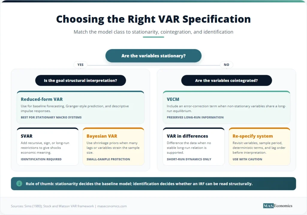
VARs also sit beside cointegration and the Engle-Granger method. A VAR in stationary variables is appropriate when the series fluctuates around stable means or has been differenced into stationarity. If non-stationary variables share a long-run equilibrium, a vector error-correction model is the correct extension. The difference is not cosmetic. A VAR in stationary inflation and unemployment studies short-run dynamics. A cointegrated system adds a long-run anchor that pulls variables back toward equilibrium.

VAR Dynamics in Matrix Form

Let \( \boldsymbol{y}_t \) be a vector containing quarterly inflation and unemployment:

where \( \pi_t \) is quarterly inflation and \( u_t \) is the unemployment rate. A two-lag reduced-form VAR is written as:

The lag operator convention is \( L y_t = y_{t-1} \). The first difference convention is \( \Delta y_t = y_t – y_{t-1} \). In this article, the VAR is written in levels for inflation and unemployment because the canonical example treats both as stationary around persistent but bounded dynamics after standard time-series checks. In applied work, the stationarity decision normally follows Augmented Dickey-Fuller testing and the broader logic explained in stationarity in time series econometrics.

The stylized coefficient matrices are:

Written equation by equation, the same system is:

The inflation equation says inflation is persistent because \( \pi_{t-1} \) and \( \pi_{t-2} \) have positive coefficients. Lagged unemployment has negative coefficients in the inflation equation, consistent with a stylized Phillips-curve pattern: higher unemployment predicts lower future inflation, holding past inflation constant. The unemployment equation is also persistent because lagged unemployment has large positive coefficients. The smaller inflation terms in the unemployment equation capture feedback from price dynamics to labour-market conditions.

The reduced-form errors \( \boldsymbol{\varepsilon}_t \) are forecast errors, not structural shocks. They are correlated because inflation and unemployment can be hit by common disturbances within the same quarter. For impulse responses, the reduced-form errors must be transformed into orthogonal shocks. In the canonical example, the structural unemployment shock is represented by the impact vector:

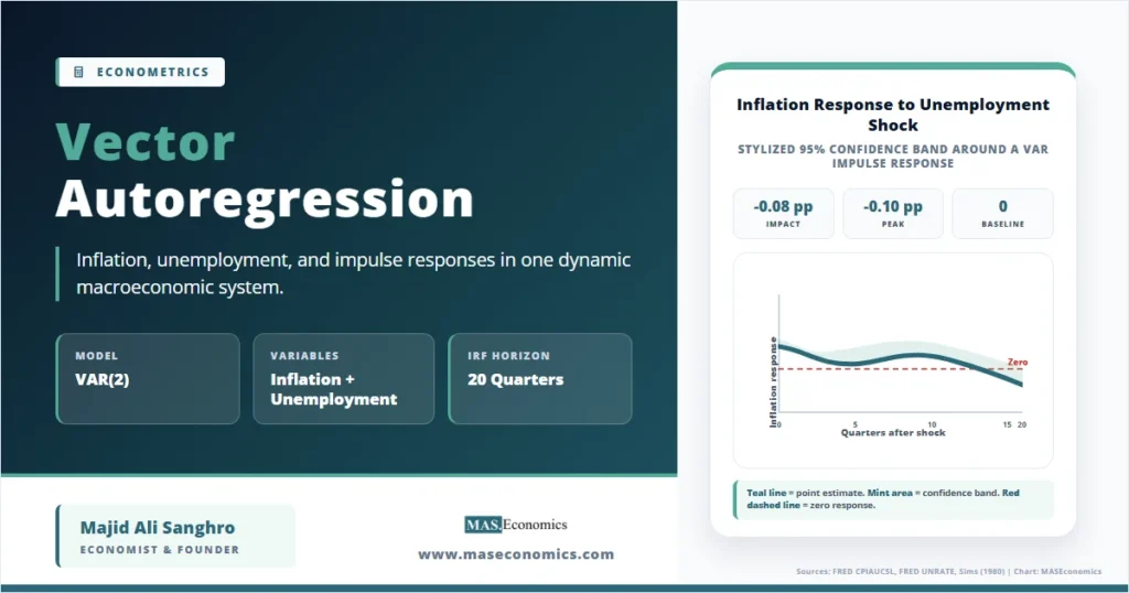
This vector means an unemployment shock raises unemployment on impact by \(0.42\) percentage points and moves inflation on impact by \(-0.08\) percentage points. The subsequent response is generated mechanically by the estimated VAR matrices:

The null and alternative hypotheses in a VAR depend on the question being asked. For predictive exclusion, the null that unemployment does not help forecast inflation is:

For impulse-response analysis, the null is usually horizon-specific. A common test asks whether the response of inflation to an unemployment shock is zero at horizon \(h\):

The decision rule compares the estimated response and its confidence band. If the 95% confidence interval excludes zero at a given horizon, the response is statistically different from zero at that horizon under the maintained model and identification scheme. If the band includes zero, the data do not reject a zero response at that horizon.

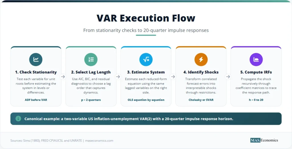
From Lag Selection to Shocks

The mathematical execution of a VAR proceeds in five steps. First, the variables are transformed so the system is suitable for estimation. Inflation is often measured as a quarterly percentage change in a price index. Unemployment is usually kept in percentage points. If a series has a unit root, differencing or a cointegrated specification is considered before fitting the VAR.

Second, the lag length \(p\) is chosen. Information criteria such as AIC and BIC compare models with different lag orders by balancing fit against parameter count. AIC tends to select richer dynamics. BIC tends to choose more parsimonious systems. The chosen lag order must be long enough to absorb residual autocorrelation, because serially correlated errors make impulse responses unreliable.

Third, each equation is estimated by ordinary least squares using the same right-hand-side variables. In a reduced-form VAR with identical regressors in every equation, equation-by-equation OLS is numerically equivalent to system least squares. This is one reason VAR estimation is straightforward even when the interpretation is not.

Fourth, the residual covariance matrix \( \boldsymbol{\Sigma} \) is estimated. This matrix contains the contemporaneous covariance of the inflation and unemployment forecast errors. Since the reduced-form residuals are usually correlated, a structural shock must be recovered using an identifying transformation. The most common baseline is a Cholesky decomposition, but the ordering of variables then matters. More structural applications use long-run restrictions, sign restrictions, or external instruments. Bernanke’s credit-channel work on the money-income correlation and Blanchard and Quah’s demand-supply decomposition show how identifying restrictions turn reduced-form dynamics into economic interpretation.

Fifth, impulse response functions are generated recursively from the estimated coefficient matrices. A one-period shock is inserted into the system. The VAR then propagates the shock forward through the lag structure. Confidence bands are usually computed by simulation, bootstrap, or asymptotic approximation. The band is not a decorative envelope. It is the inference object that separates a visible line from an estimated response that is statistically distinguishable from zero.

Reading the IRF: Inflation After an Unemployment Shock

The stylized canonical example estimates a quarterly VAR(2) for US inflation and unemployment. The table reports the coefficient matrix in journal format. Each column is an equation. Each row is a lagged regressor. Coefficients appear first, with standard errors directly below in parentheses.

Table 1. VAR Estimation: US Inflation and Unemployment

Regressor	Inflation equation \( \pi_t \)	Unemployment equation \( u_t \)
Constant	0.18**	0.09
	(0.07)	(0.06)
\( \pi_{t-1} \)	0.52***	0.05
	(0.10)	(0.07)
\( u_{t-1} \)	-0.08*	0.71***
	(0.04)	(0.08)
\( \pi_{t-2} \)	0.21**	-0.02
	(0.09)	(0.06)
\( u_{t-2} \)	-0.04	0.18**
	(0.03)	(0.07)
Lag order	2 quarters
Observations	168 quarterly observations
AIC	-1.42
BIC	-1.18
Residual correlation	-0.34

Note: ^* p<0.10, ^** p<0.05, ^*** p<0.01. Standard errors in parentheses. Stylized canonical example based on quarterly US inflation and unemployment dynamics.

The inflation equation contains two important pieces of information. Inflation persistence is strong because the first lag of inflation is 0.52 and the second lag is 0.21. Lagged unemployment enters with a negative sign, meaning higher unemployment predicts lower inflation in later quarters. The first unemployment lag is marginally different from zero, while the second unemployment lag is not individually precise. The system still matters because VAR interpretation is not limited to one coefficient. The full dynamic effect combines both lag matrices and the covariance structure of the shocks.

The unemployment equation is highly persistent. The first unemployment lag is 0.71 and the second lag is 0.18. The inflation terms in that equation are small. This does not mean inflation is irrelevant for unemployment in every economic sense. It means that, in this stylized reduced-form system, unemployment mostly forecasts itself once the lagged system is included.

The impulse response function converts the coefficient matrix into a dynamic path. The chart below shows the response of inflation to a one-standard-deviation unemployment shock. The point estimate is negative on impact and remains below zero for several quarters. The 95% band excludes zero during the middle horizons, then includes zero as the response fades.

The correct reading begins at horizon zero. The unemployment shock has an immediate negative effect on inflation of \(-0.080\) percentage points. At horizon one, the response is \( \mathbf{A}_1\boldsymbol{s}_u \), giving \(-0.075\) percentage points for inflation. By horizon four, the response is about \(-0.104\) percentage points. The effect then decays slowly because both inflation and unemployment are persistent. By horizon twenty, the response is close to zero.

The economic interpretation is not that unemployment mechanically lowers inflation in every episode. The interpretation is conditional on the identification scheme and the VAR specification. In this stylized system, an unemployment shock looks like a demand-side cooling episode: slack rises, inflation declines, and the effect fades gradually. A supply shock would require a different structural interpretation and might move inflation and unemployment in the same direction.

The inference comes from the confidence band. During horizons two through seven, the upper band is near or below zero, so the estimated negative response is statistically meaningful under the model. At longer horizons, the band includes zero. The data then fail to reject a zero response, even though the point estimate remains slightly negative. In applied macroeconometrics, that distinction is key. The line tells the estimated path. The band tells how much uncertainty surrounds the path.

Where VAR Identification Breaks Down

A VAR can fail even when its equations look statistically tidy. The first failure is non-stationarity. If the variables contain unit roots and are not cointegrated, a levels VAR can confuse shared trending behaviour with dynamic relationships. Differencing may solve the statistical problem, but remove long-run information. Cointegration changes the model class because the correct specification becomes a vector error-correction model.

The second failure is overfitting. A VAR with \(k\) variables and \(p\) lags estimates many parameters. Each additional variable adds an equation, and each extra lag adds a full coefficient matrix. In small samples, a large VAR can fit historical noise and produce unstable impulse responses. This is one reason Bayesian VARs and shrinkage methods became common in forecasting institutions.

The third failure is weak identification. A recursive Cholesky ordering imposes a contemporaneous causal sequence. If unemployment is ordered after inflation, the model says inflation can affect unemployment within the quarter, while unemployment affects inflation only with a delay. Reversing the order changes the structural shocks. When the ordering is arbitrary, the IRF becomes a property of the assumption rather than a robust empirical finding.

The fourth failure is structural instability. Macroeconomic relationships can change across monetary-policy regimes, crises, and data revisions. The BIS paper Can VARs describe monetary policy? discusses the difficulty of using reduced-form VARs for monetary-policy analysis when the policy rule and private-sector behaviour shift over time. A VAR estimated over a long sample may average across regimes that should not be pooled.

How Central Banks Use VARs to Forecast Policy Effects

Central banks use VARs because monetary policy works through lagged, interdependent channels. Inflation, unemployment, output, interest rates, exchange rates, and credit conditions respond to each other over time. A policy-rate shock does not move one variable in isolation. It changes financial conditions, demand, labour-market slack, and price-setting behaviour. VARs provide a disciplined way to trace those dynamic responses.

In policy work, the VAR is rarely the only model. It sits beside structural macro models, judgmental forecasts, market-based expectations, and sectoral data. Its value comes from transparency. A VAR can show how a historical monetary-policy shock has typically affected output and inflation over several quarters. It can also show whether the estimated effect is precise or surrounded by wide uncertainty.

The Federal Reserve’s framework explicitly combines price stability and maximum employment, described in its monetary policy review and assessment. A VAR built around inflation and unemployment is therefore not an abstract statistical exercise. It mirrors the dual variables that dominate central-bank reaction functions. The next natural link is the Taylor Rule reaction function, where policy rates respond systematically to inflation gaps and output or unemployment gaps. Once that central-banking article is updated, it should link forward to VARs as the empirical tool for tracing policy shocks through time.

VARs also connect to the MASEconomics time-series cluster. ARMA models and forecasting explain persistence in a single series. Multivariate time series models extend that logic to systems. autocorrelation in time series econometrics explains why residual dependence must be handled before inference is trusted. econometric model selection gives the information-criterion logic behind lag choice.

The applied literature also shows why VARs must be read carefully. Sims introduced VARs as a response to heavily restricted macroeconometric models. Bernanke used VAR-style evidence to compare monetary and credit interpretations of the money-income correlation. Blanchard and Quah used long-run restrictions to separate demand and supply disturbances. Stock and Watson later presented VARs as one of the core tools for empirical macroeconomics, especially for forecasting and dynamic analysis.

The modern lesson is balanced. VARs are strong descriptive systems and useful forecasting devices. They are also fragile structural tools unless identification is explicit. A central bank can use a VAR to ask what usually happens after a tightening shock, how long inflation takes to respond, and how much unemployment rises along the estimated path. The answer remains conditional on the model, not a mechanical law of policy.

MASEconomics Explains

Conclusion

Vector autoregression is the standard system-based framework for studying dynamic relationships among macroeconomic variables when theory does not supply enough credible single-equation restrictions. A VAR places each variable in the system on equal footing, estimates lagged cross-dependence, and uses impulse response functions to trace the effect of identified shocks through time. In the US inflation-unemployment example, a positive unemployment shock produces a negative inflation response that fades gradually, with the strongest evidence appearing in the early and middle horizons. The model is powerful because it respects macroeconomic feedback. Its interpretation remains conditional on stationarity, lag choice, sample stability, and identification.

Thanks for reading! If you found this helpful, share it with friends and spread the knowledge. Happy learning with MASEconomics