Granger Causality: Predictive Order in Time Series

In weekly fuel markets, crude oil prices often move before retail gasoline prices. That timing pattern is exactly where Granger Causality enters econometrics: it tests whether past values of one time series contain useful information for forecasting another time series after the target variable’s own history has already been included.

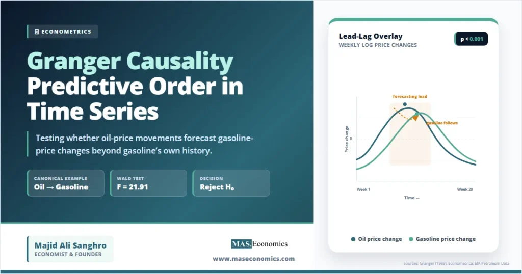
The method is not a claim about deep structural causation. It is a disciplined test of predictive order. In the canonical oil-to-gasoline case, the economic question is whether lagged oil-price changes help forecast gasoline-price changes beyond gasoline’s own lagged movements. That distinction matters because many macroeconomic and financial variables move together, yet only some carry independent forecasting content.

Predictive Order in Fuel Markets

Retail gasoline prices are built from crude oil costs, refining margins, distribution costs, marketing costs, taxes, and local supply conditions. The U.S. Energy Information Administration states that crude oil is usually the largest component of retail gasoline prices, and its share changes over time and across regions. In January 2026, EIA’s gasoline price breakdown placed crude oil at 51 percent of the U.S. regular gasoline price, with refining, taxes, and distribution making up the rest through the fuel supply chain.

That institutional relationship gives the Granger test a natural setting. If crude oil is an upstream input, oil prices should carry predictive information about later gasoline prices. But the test still has to prove this statistically. Gasoline prices also have their own inertia. Retail prices may adjust slowly because inventories, contracts, taxes, local competition, and refinery bottlenecks all affect the pace of pass-through.

The Dallas Fed’s research on crude oil and gasoline prices used time-series methods, including Granger causality, to study where petroleum price shocks originate and how they move through the market. That is the right framing. The test does not say that an oil shock is the only cause of gasoline prices. It asks whether past oil-price movements improve forecasts of gasoline prices once gasoline’s own past has already been taken seriously.

This makes Granger causality a bridge between descriptive correlation and structural causal analysis. Simple correlation says two series move together. Ordinary regression may say gasoline prices rise when oil prices rise. Granger causality asks a sharper time-series question: do lagged oil prices improve the forecast of gasoline prices beyond lagged gasoline prices alone?

The same logic appears across macroeconomics. Inflation expectations may forecast inflation. Interest-rate spreads may forecast recessions. Money growth may forecast oil prices in some regimes, as explored in the IMF paper on Granger predictability of oil prices. Central banks and research institutions use these lead-lag tests because forecasting systems need to know which variables add independent information and which merely repeat information already contained elsewhere.

Forecasting Content in Equations

Clive W. J. Granger’s original 1969 paper, “Investigating Causal Relations by Econometric Models and Cross-Spectral Methods”, defined causality in terms of improved prediction. If the past of \(x_t\) helps predict \(y_t\), after all relevant past information has been included, then \(x_t\) is said to Granger-cause \(y_t\).

For the oil-to-gasoline example, let \(g_t\) denote the weekly change in the log gasoline price and \(o_t\) denote the weekly change in the log crude oil price. The unrestricted two-lag model is:

The restricted model removes the lagged oil terms:

The null hypothesis is that lagged oil-price changes do not improve forecasts of gasoline-price changes:

The alternative hypothesis is that at least one lagged oil coefficient is different from zero:

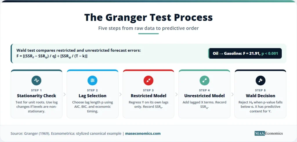
A Wald test compares the unrestricted model with the restricted model. In an \(F\)-test version, the statistic can be written as:

Here \(SSR_r\) is the sum of squared residuals from the restricted model, \(SSR_u\) is the sum of squared residuals from the unrestricted model, \(q\) is the number of restrictions, \(T\) is the number of observations, and \(k\) is the number of parameters estimated in the unrestricted equation.

For the stylized canonical example, suppose the restricted gasoline-only model has \(SSR_r = 0.0450\), the unrestricted oil-plus-gasoline model has \(SSR_u = 0.0384\), the number of restrictions is \(q = 2\), weekly observations are \(T = 260\), and the unrestricted equation estimates \(k = 5\) parameters. The resulting statistic is:

With two numerator restrictions and 255 denominator degrees of freedom, an \(F\)-statistic of 21.91 implies a p-value below 0.001. The null is rejected. In this stylized example, lagged oil-price changes Granger-cause gasoline-price changes.

The reverse direction can also be tested by placing oil-price changes on the left-hand side and asking whether lagged gasoline-price changes forecast oil-price changes:

The reverse null is \(H_0: \delta_1 = \delta_2 = 0\). If that null is not rejected, the evidence points to one-way predictive ordering: oil prices lead gasoline prices, but gasoline prices do not lead oil prices. If both nulls are rejected, the system has feedback. If neither null is rejected, the two series may move together without useful short-run predictive content in either direction.

How the Wald Test Computes

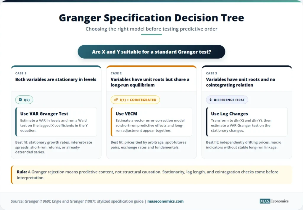
The algorithm starts by making the series suitable for time-series regression. Many energy prices are non-stationary in levels, so the test is usually applied to log changes or returns unless a cointegrating relationship justifies a vector error-correction model. This connects directly to the Augmented Dickey-Fuller Test and stationarity in time series econometrics. A Granger test on trending levels can produce misleading results because both series may share broad movement without genuine forecasting content.

Next comes lag selection. A two-lag weekly model says that the previous two weeks of oil-price changes and gasoline-price changes are allowed to affect the current gasoline-price change. Longer lag lengths can be selected by information criteria such as AIC or BIC, which are discussed in econometric model selection. Too few lags leave autocorrelation in the residuals. Too many lags reduce power because the model estimates unnecessary parameters.

The unrestricted model is estimated first. The regression includes gasoline’s own lags and oil’s lags. The restricted model is estimated next by forcing the oil-lag coefficients to zero. The Wald test then asks whether the drop in residual variation from adding oil lags is large enough relative to the model’s remaining unexplained variation. The larger the improvement, the larger the test statistic.

Modern vector autoregression software implements the same logic in system form. The statsmodels VAR causality documentation describes the null as no Granger causality from one variable or group of variables to the remaining variables in the system. The mathematics is still a joint restriction test on lagged coefficients. The software should never be the explanation. The explanation is the comparison between the restricted and unrestricted forecasting equations.

Finally, the decision rule is simple. If the p-value is below the chosen significance level, reject the null of no Granger causality. If the p-value is above the chosen significance level, fail to reject the null. Failure to reject does not prove the absence of economic influence. It means the available lags, data frequency, sample period, and model specification do not show enough independent forecasting content.

Reading the Granger-Wald Test

The stylized output below follows the oil-to-gasoline canonical example. The left-hand-side variable is weekly gasoline-price growth, measured as \(g_t = \Delta \ln(G_t)\). The main question is whether lagged weekly oil-price growth improves gasoline forecasts after two gasoline lags are already included.

Table 1. Granger Wald Test: Oil Prices and Gasoline Prices

Test Direction	Null Hypothesis	Wald F-statistic	p-value	Decision
Oil → Gasoline	Lagged oil changes do not forecast gasoline changes	21.91***	<0.001	Reject \(H_0\): oil Granger-causes gasoline
Gasoline → Oil	Lagged gasoline changes do not forecast oil changes	1.24	0.291	Fail to reject \(H_0\): no reverse predictive content
Lag length	Weekly lags included in each equation	2	AIC-selected	Short-run pass-through window
Restricted SSR	0.0450
Unrestricted SSR	0.0384
Observations	260 weekly observations

Note: ^* p<0.10, ^** p<0.05, ^*** p<0.01. Stylized canonical example. The table reports a Wald test on two lagged coefficients in each direction.

The first row rejects the null. Lagged oil-price changes contain useful forecasting information for gasoline-price changes. The second row fails to reject the reverse null. Lagged gasoline-price changes do not carry the same predictive content for oil-price changes. The direction is consistent with an upstream-input interpretation: crude oil leads the retail fuel chain.

The result is economic, not merely statistical. Gasoline is refined from crude oil and other petroleum liquids, as explained in the EIA’s gasoline overview. Oil-price changes enter refinery economics before they appear fully in retail gasoline prices. That supply-chain timing creates a plausible lead-lag structure. The test then measures whether the lead is visible in the data.

The chart below visualizes the same stylized pattern. The oil-price change series leads. The gasoline-price change series follows with a short delay. The visual relationship does not replace the Wald test, but it helps explain why the test rejects the oil-to-gasoline null.

Where Predictive Causality Breaks

Granger causality is powerful because it has a clear decision rule. It is fragile because the decision depends on specification. The first failure point is non-stationarity. If oil prices and gasoline prices are tested in levels while both contain unit roots, the regression can detect shared trends rather than genuine forecasting content. The safer approach is to test stationarity first, use log changes when appropriate, and consider cointegration methods when non-stationary series share a long-run equilibrium.

The second failure point is omitted-variable timing. Suppose refinery outages, seasonal driving demand, exchange rates, shipping disruptions, and tax changes all affect gasoline prices. A bivariate oil-gasoline test may attribute too much forecasting content to oil because oil is correlated with omitted forces. A multivariate test inside a VAR can reduce this risk by adding relevant controls, but it cannot eliminate every omitted shock.

The third failure point is lag length. A one-week lag may miss slow pass-through. A twelve-week lag may dilute the test by adding many weak parameters. Information criteria help, but economic reasoning still matters. Gasoline-price pass-through may be faster in wholesale markets than in retail markets. It may also change during crises, refining outages, or periods of price controls.

The fourth failure point is instability. Energy markets change when shale production expands, refinery capacity tightens, geopolitical risk rises, or taxes shift. A Granger relationship estimated over one period may weaken in another. The ECB working paper on Granger-causal priority and variable choice in VAR models shows why variable ordering and predictive priority matter in multivariate systems. The result is not a timeless law. It is a sample-specific statement about predictive information.

The fifth failure point is confusing Granger causality with causal inference. A randomized experiment, natural experiment, instrumental variable strategy, or structural model can support stronger causal claims than a lead-lag test. The MASEconomics article on causal inference in economics explains why causal identification requires more than forecasting success. Granger causality belongs in the forecasting and dynamic-modeling toolkit, not as a substitute for identification design.

Energy Forecasting and Policy Models

Granger causality is widely used because modern macroeconomics is full of dynamic systems. Oil prices affect inflation, transport costs, household budgets, and external balances. Exchange rates affect import prices and debt-service costs. Interest rates affect credit, housing, and investment with lags. These relationships are rarely instantaneous, so time ordering becomes part of the economic evidence.

Energy markets provide a clear example. The EIA publishes weekly and daily petroleum price data because energy-price movements are transmitted through refineries, wholesale contracts, inventories, and retail markets. The EIA daily prices page tracks crude oil, gasoline, heating oil, diesel, and crack spreads. A Granger-style system can test whether one part of that chain leads another. Oil-to-gasoline causality supports the idea of upstream pass-through. Gasoline-to-oil causality would suggest feedback from downstream demand conditions into upstream pricing.

Central banks care about these dynamics because energy shocks can move headline inflation before core inflation responds. A VAR system can include oil prices, gasoline prices, inflation, output, and interest rates, and then test predictive links among them. Granger causality is often an entry point into larger tools such as multivariate time series models and vector autoregression. VARs extend the same logic by treating every variable as potentially endogenous and by tracing shock transmission through impulse responses.

The relationship with ARMA models and forecasting is also direct. ARMA models use a variable’s own past and past shocks to forecast itself. Granger causality asks whether another variable’s past adds information beyond that self-history. In this sense, the test is a formal contest between an autoregressive forecast and an expanded dynamic forecast.

For applied forecasting teams, the test can simplify model design. If oil prices do not Granger-cause gasoline prices after other variables are included, the model may not need oil lags for that forecasting horizon. If oil prices strongly Granger-cause gasoline prices, dropping oil lags would throw away useful information. This logic is also why the test appears in work on inflation expectations, exchange rates, commodity prices, asset returns, and macro-financial linkages.

The method also clarifies the limits of forecasting. A Granger relationship can disappear when policy regimes change. Fuel taxes, refinery capacity, strategic reserves, or trade disruptions can alter pass-through. A strong pre-crisis relationship may fail during a crisis because constraints move from ordinary input costs to physical supply bottlenecks. Good applied econometrics, therefore, combines statistical testing with institutional knowledge.

The oil-to-gasoline example fits the broader MASEconomics econometrics sequence. The econometrics foundation explains how theory and data interact. Simple regression and multiple regression explain conditional association. ADF testing handles stationarity. Granger causality then adds dynamic predictive ordering. VARs and cointegration models extend the framework to richer systems.

MASEconomics Explains

Conclusion

Granger Causality gives econometrics a rigorous way to test predictive order in time-series data. In the oil-to-gasoline example, the method compares a gasoline-only forecast with a forecast that also includes lagged oil-price changes. If the added oil lags reduce forecast errors enough to reject the joint null, oil prices Granger-cause gasoline prices in the predictive sense.

The test is most useful when it is treated with discipline. Stationarity must be checked, lag length must be justified, omitted variables must be considered, and the result must not be overstated as structural causation. Within those limits, Granger causality is one of the cleanest tools for identifying whether one time series leads another in a statistically meaningful forecasting system.

The test is most useful when it is treated with discipline. Stationarity must be checked, lag length must be justified, omitted variables must be considered, and the result must not be overstated as structural causation. Within those limits, Granger causality is one of the cleanest tools for identifying whether one time series leads another in a statistically meaningful forecasting system.

Thanks for reading! If you found this helpful, share it with friends and spread the knowledge. Happy learning with MASEconomics