Deadweight Loss: Welfare Cost of Market Distortions

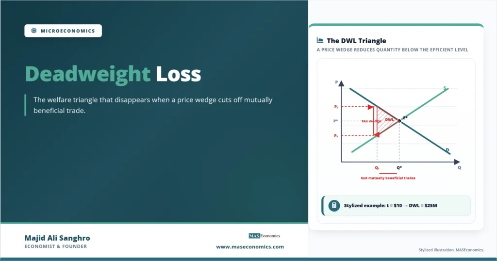
When a US administration places a 25 percent tariff on imported steel, the customs revenue collected by the Treasury is easy to count. What rarely makes the headlines is the smaller second number sitting next to it: the value of trades that simply do not happen because the tariff has pushed the buyer and the seller far enough apart that neither finds the deal worth completing. That uncounted loss is the focus of one of the most useful diagrams in microeconomics. The deadweight loss triangle is the area where mutually beneficial trade has been switched off by a price wedge, and it appears in nearly every analysis of taxes, tariffs, price controls, monopolies, and externalities.

The triangle itself is defined by its base, the reduction in equilibrium quantity, and its height, the size of the wedge. The Harberger formula ties the welfare cost to the square of the tax rate and the elasticities of demand and supply. The same geometric logic explains the efficiency loss from price floors, monopoly pricing, and externalities, making the diagram the shared language of applied welfare analysis across microeconomics.

Mutual Gains and Foregone Trade

A competitive market without distortions produces a particular outcome: every unit for which the buyer’s willingness to pay exceeds the seller’s marginal cost gets produced and sold. The intersection of supply and demand curves is not just where price clears; it is also the quantity at which the last unit traded creates exactly zero additional surplus. Pushing past that quantity would force units onto the market for which the cost exceeds the value. Stopping short of it leaves potential gains on the table.

Consumer surplus is the area between the demand curve and the price line, summing the difference between what each buyer would have paid and what each buyer actually paid. Producer surplus is the area between the price line and the supply curve, summing the difference between the price received and the marginal cost of production. Together they form the total surplus that the market generates. At the competitive equilibrium, this combined area reaches its maximum. Any policy or market structure that changes the traded quantity away from that point will shrink it.

Deadweight loss is the size of that shrinkage. It is the slice of surplus that simply disappears: it does not transfer from consumers to producers, from producers to the government, or from sellers to monopolists. It vanishes because the trades that would have produced it never take place. This is what gives the concept its weight in policy analysis. Tax incidence debates often focus on who pays the tax, but the deadweight triangle measures what no one collects.

Anatomy of the Tax Triangle

Consider a per-unit tax of t placed on a good. Buyers see a higher price, sellers receive a lower price, and the difference between the two is the tax wedge. The quantity traded falls from the no-tax equilibrium Q* to a smaller quantity Q_t. Geometrically, the deadweight loss is the triangle bounded above by the demand curve, below by the supply curve, and on the left by the new lower quantity.

Three things change with the tax. First, consumer surplus shrinks because buyers who still purchase pay Pb instead of P*, and some buyers exit the market entirely. Second, producer surplus shrinks because sellers who still produce receive P_s instead of P*, and some output disappears. Third, the government collects revenue equal to t × Q_t, which corresponds to the rectangle bounded by the two prices and the new quantity.

The lost surplus that does not flow into government revenue is exactly the triangle. Its base is the reduction in quantity, Q* − Q_t. Its height is the tax wedge, t. Its area is the standard triangle formula:

Deadweight Loss From a Tax

Where t is the per-unit tax and ΔQ is the reduction in equilibrium quantity. Linearity is assumed locally.

The formula carries a useful implication. Doubling the tax does not double the deadweight loss; it roughly quadruples it. The base of the triangle grows with the wedge, and the height grows with the wedge, so the area scales with the square. This is the basic mathematical reason why economists generally prefer broad-based taxes with low rates over narrow taxes with high rates: a small wedge applied to a large base produces less aggregate distortion than a large wedge applied to a small base.

Elasticities and the Size of the Triangle

The reduction in quantity, ΔQ, is not a fixed number. It depends on how responsive buyers and sellers are to price changes. A tax of the same size produces a much smaller triangle in a market where quantities barely move than in a market where small price changes drive large quantity shifts. This is where price elasticity moves from a definition exercise into a welfare instrument.

Arnold Harberger formalized this relationship in his 1964 study of taxation, deriving an approximation that links deadweight loss to elasticities and the tax rate. For a small tax in a market with linear demand and supply, the welfare cost can be written as:

Harberger Approximation

Where τ is the tax as a fraction of price, ε_D and ε_S are the absolute values of the demand and supply elasticities, and P and Q are the pre-tax equilibrium values.

Two features of this expression are worth pausing on. The tax rate enters as a square, confirming that small taxes are disproportionately less distortionary than large ones. The elasticities enter through a harmonic-mean structure, which means the smaller of the two dominates. If supply is highly inelastic, a tax on the good will mostly translate into a lower price received by sellers rather than a quantity reduction, and the deadweight loss stays small. The same logic applies to inelastic demand.

This is the technical foundation for the old Ramsey rule on optimal commodity taxation: tax goods with low elasticities more heavily than goods with high elasticities, holding revenue requirements fixed. Real tax systems rarely follow Ramsey directly because of equity considerations, since necessities are often the most inelastic goods. But the welfare logic is robust, and it explains why excise taxes on cigarettes, alcohol, and gasoline raise substantial revenue with modest deadweight loss compared with broad-based consumption taxes at similar rates.

The Triangle Across Other Distortions

The same geometric pattern appears across very different policy contexts. Once the demand-supply diagram is in hand, the deadweight triangle becomes a transferable tool.

A binding price ceiling, such as rent control set below the market-clearing rent, holds the price below P*. At the lower price, the quantity supplied falls below the quantity demanded. The traded quantity is determined by the short side of the market, which is supply. The deadweight triangle sits between the supply curve and the demand curve from the constrained quantity back to Q*, and it captures the surplus that would have been created by tenants and landlords who would have transacted at intermediate prices but cannot under the ceiling. A binding price floor, such as a minimum wage set above the market-clearing wage, produces the symmetric picture on the labor side, with employment below the competitive level and a triangle of foregone employment relationships.

A monopoly producer with market power restricts output below the competitive level to drive price up the demand curve. The firm chooses the quantity where marginal revenue equals marginal cost, not where price equals marginal cost. The result is the same kind of triangle, this time bounded by the demand curve above, the marginal cost curve below, and the gap between the monopoly quantity and the competitive quantity to the right. The monopolist captures additional profit as a rectangle, but the triangle is pure loss. This is one of the central results of the analysis of different market structures, and it is why antitrust enforcement targets restrictions on output rather than just high prices.

A negative externality, such as pollution, drives a wedge between private cost and social cost. The private market produces where private marginal cost meets demand, but the socially efficient quantity sits where social marginal cost meets demand. The deadweight loss in this case is the area between the social marginal cost curve and the demand curve, from the efficient quantity back to the private equilibrium quantity. It represents the value of the harm imposed on third parties, net of the value created by the additional units of output. This is the welfare logic that underpins market failure analysis and the case for Pigouvian taxes.

A tariff on imports produces two deadweight triangles in the importing country: a production-side triangle from inefficient domestic firms producing units that could have been imported more cheaply, and a consumption-side triangle from buyers priced out of the market. The customs revenue and the gain to domestic producers are transfers, but the two triangles are deadweight losses. In a small open economy, these triangles are the full welfare cost. In a large economy, terms-of-trade effects can offset part of the loss, which is the subject of the optimal-tariff literature.

A Worked Numerical Example

Suppose the market for a good has linear inverse demand P = 100 − Q and linear inverse supply P = 20 + Q, with quantities measured in millions of units and prices in dollars. Setting supply equal to demand gives the competitive equilibrium: Q* = 40, P* = 60. Total surplus at the no-tax equilibrium is the area of the large triangle between the two curves, which works out to $1,600 million.

A per-unit tax of t = 10 shifts the wedge between buyer and seller prices to ten dollars. Solving the system, the new quantity becomes Q_t = 35, the buyer pays P_b = 65, and the seller receives P_s = 55. Government revenue is 10 × 35 = $350 million. The deadweight loss is ½ × 10 × 5 = $25 million.

Table 1. Welfare Accounting Before and After a Per-Unit Tax of $10

Welfare Component	No Tax	With Tax (t = 10)	Change
Consumer Surplus	800	612.5	−187.5
Producer Surplus	800	612.5	−187.5
Government Revenue	0	350.0	+350.0
Total Surplus	1,600	1,575.0	−25.0
Deadweight Loss	0	25.0	+25.0
Source: Stylized example based on standard formulas.

The accounting makes the geometry concrete. Consumers and producers each lose $187.5 million in surplus. Of that combined $375 million, the government recovers $350 million as revenue. The remaining $25 million is the triangle. It is the value of trades between buyers willing to pay between $55 and $65 and sellers willing to accept the same range, none of which now happens because the tax wedge has made those deals jointly unprofitable.

Doubling the tax to t = 20 produces a new quantity of 30, a $100 million deadweight loss, and revenue of $600 million. The tax doubled, the revenue did not quite double, and the deadweight loss quadrupled. This is the square-of-the-rate result visible in arithmetic.

The deadweight triangle is sensitive to where it sits on the curves. A small tax near the equilibrium produces a thin triangle. The same tax applied in a steeply sloped section of demand or supply, where elasticities are low, produces a much smaller triangle than in a flat section, where elasticities are high. The size of the wedge is only half the story.

Limitations of the Diagram

The deadweight loss triangle is one of the most useful diagrams in microeconomics, but it operates under assumptions that are worth keeping in view.

The triangle measures static efficiency loss in a partial equilibrium frame. It treats the market for one good in isolation, holding incomes, the prices of other goods, and aggregate production capacity fixed. In general equilibrium, taxes interact with other distortions. A tax that reduces deadweight loss in one market may worsen it in another, and the welfare accounting of welfare economics at the economy-wide level is more nuanced than the single-market triangle suggests. This is the substance of the theory of the second best: in a world with multiple existing distortions, removing one of them does not automatically improve welfare.

The triangle also rests on competitive benchmarks. It compares the distorted outcome with the perfectly competitive equilibrium and treats any deviation as a loss. When the competitive benchmark itself is not attainable, because of market power, information problems, or transaction costs, the relevant comparison may be between two imperfect outcomes rather than between a distortion and a frictionless ideal. In such cases, the geometric loss is a useful upper bound rather than a literal welfare cost.

Equity considerations sit outside the triangle entirely. A tax that produces a small deadweight loss may still be objectionable on distributional grounds, and a regulation that produces a large efficiency loss may be defended on the basis of fairness, paternalism, or political values that the diagram cannot weigh. Welfare economics does not pretend to settle these arguments; it just provides the efficiency cost as one input to them.

Empirical Estimates and Policy Stakes

The triangle is a teaching device, but the elasticities and the rates that feed it are real, and economists have spent decades measuring deadweight loss in actual tax systems. Harberger’s original 1964 estimate of the welfare cost of US corporate income taxation came in at roughly half a percent of national income. Martin Feldstein’s later work, which incorporated the response of taxable income to marginal rates rather than just hours worked, produced substantially larger estimates that influenced the optimal-taxation literature through the 1980s and 1990s. Studies of payroll taxes, value-added taxes, and capital-income taxes by the Congressional Budget Office and the OECD have produced ranges depending on the elasticities assumed and the tax interactions considered.

The policy implications run in several directions. Tax systems should aim for broad bases and low rates to keep the wedge small. Excise taxes on inelastic goods, sometimes justified on externality grounds, carry a low deadweight cost. Marginal income tax rates faced by high earners, where labor supply or taxable income elasticities are higher, generate larger deadweight loss per dollar of revenue, which is the empirical content of Laffer-curve arguments without the rhetorical excesses. Tariffs in small economies are essentially pure deadweight loss instruments, since the revenue collected is generally smaller than the welfare cost. Price controls in housing and labor markets carry a deadweight component whose size depends on the elasticities of supply, which is why economists tend to prefer income transfers over price interventions when the goal is to help low-income households.

Explains

Conclusion

The deadweight loss triangle is a small piece of geometry that carries a large amount of economic reasoning. It identifies the surplus that does not transfer but simply disappears when a market distortion drives a wedge between the price buyers pay and the price sellers receive. Its base is the reduction in quantity, its height is the wedge, and its area scales with the square of the distortion. The triangle reappears across taxes, tariffs, price controls, monopoly pricing, and externalities, which is why it sits near the center of welfare analysis in microeconomics.

The diagram is most useful when its assumptions are remembered. It measures static efficiency loss in a single market under competitive benchmarks. Real economies have multiple interacting distortions, second-best considerations, equity concerns, and dynamic effects that the triangle cannot capture. None of this diminishes the tool. The competitive benchmark and the triangle that measures deviations from it are the starting point for almost every applied welfare analysis in economics, from optimal taxation to antitrust enforcement to the design of environmental policy. The arithmetic is simple, but what it reveals about the cost of interfering with mutually beneficial trade is not.

Frequently Asked Questions

Thanks for reading! If you found this helpful, share it with friends and spread the knowledge. Happy learning with MASEconomics