The Price Elasticity of Demand and Supply

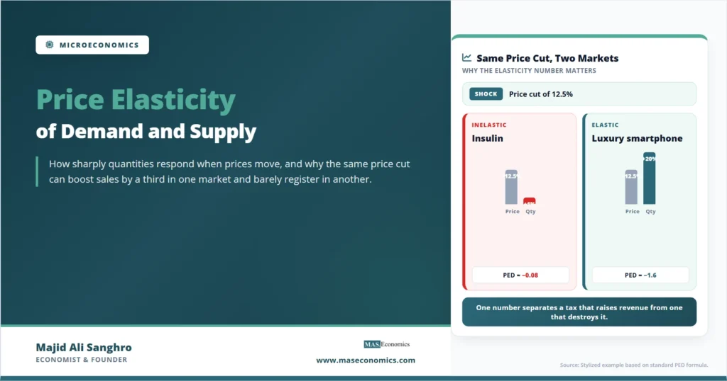
When the UK government cut fuel duty by 5 pence per liter in March 2022, the first change to fuel duty rates in 11 years, pump prices fell briefly by less than the full 5 pence, then resumed climbing. By July of the same year, petrol prices reached a record 191.6 pence per liter, and consumption remained largely unchanged through the entire episode. When Apple cut the iPhone SE price by 17 percent in early 2024, unit sales jumped by more than a third within a quarter. Two price cuts, two completely different responses. The concept that explains this is the price elasticity of demand and supply, which measures how sharply quantities respond when prices move. It is one of the most-used numbers in applied economics, sitting behind tax policy, pricing strategy, agricultural planning, and central-bank assessments of pass-through.

The intuition is simple. In a market for supply and demand, quantity demanded falls when price rises, and quantity supplied rises when price rises. Those are directional facts. Elasticity adds the missing piece: the magnitude. By how much does quantity move when price moves one percent? The answer to that question separates an essential commodity from a luxury, a fast-adjusting factory from a slow-adjusting farm, and a tax that raises revenue from a tax that mostly destroys it.

What Elasticity Measures

Elasticity is a unit-free measure of responsiveness. It is calculated as the percentage change in one variable divided by the percentage change in another. Because both numerator and denominator are in percentages, the units cancel. An elasticity of 1.5 means the same thing whether the underlying market is wheat priced in dollars per bushel or smartphones priced in rupees per unit.

The two elasticities covered in this article both involve price. Price elasticity of demand asks how much the quantity demanded responds to a change in the good’s own price. Price elasticity of supply asks the same question on the production side. Other elasticities exist, including cross-price elasticity (response to the price of a different good) and income elasticity (response to consumer income), and these are covered in separate articles linked at the end.

The standard size convention is to read elasticities in absolute value when categorizing them as elastic or inelastic, even though price elasticity of demand is mathematically negative by construction.

Table 1. Price Elasticity of Demand and Supply at a Glance

Measure	Formula	Typical sign	Categorization	Stylized example
Price Elasticity of Demand (PED)	\( PED = \dfrac{\%\Delta Q_d}{\%\Delta P} \)	Negative	Elastic if |PED| > 1; Inelastic if |PED| < 1; Unit elastic if |PED| = 1	Luxury smartphones: PED ≈ −1.6
Price Elasticity of Supply (PES)	\( PES = \dfrac{\%\Delta Q_s}{\%\Delta P} \)	Positive	Elastic if PES > 1; Inelastic if PES < 1; Unit elastic if PES = 1	Smartphones: PES ≈ 2.5; Wheat: PES ≈ 0.25
Source: MASEconomics editorial synthesis. Example values are illustrative.

Price Elasticity of Demand

Price elasticity of demand (PED) measures how the quantity demanded of a good responds to a change in its own price. Formally:

PRICE ELASTICITY OF DEMAND

The value is typically negative because of the inverse relationship between price and quantity demanded. Economists usually interpret it in absolute value.

Consider a worked example. A luxury smartphone brand drops its flagship price from $800 to $700, a 12.5 percent reduction. Quantity demanded rises from 1,000 units to 1,200 units, a 20 percent increase. The PED is:

The absolute value of 1.6 indicates elastic demand: a one percent price cut produced roughly 1.6 percent more sales. The buyer base for this product is highly price-responsive, which is consistent with most luxury electronics, where alternatives are plentiful.

The standard categorization works as follows. Elastic demand carries an absolute PED greater than one, meaning a price change produces a larger proportional change in quantity. Inelastic demand carries an absolute PED below one, meaning quantity barely moves when price moves. Unit elastic demand sits at exactly one, where percentage changes match. Two extreme cases bookend the range: perfectly inelastic demand at PED equal to zero (a life-saving medication where quantity does not change at all with price), and perfectly elastic demand at PED approaching infinity (a homogeneous commodity where any price above the market level loses all sales).

The image below visualizes the slope difference between elastic and inelastic demand curves.

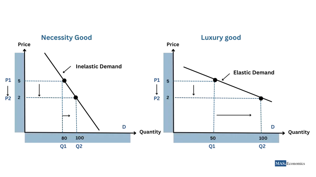
The steeper demand curve represents an inelastic good, such as a necessity. The flatter demand curve represents an elastic good, such as a luxury or a good with close substitutes. The slope difference is not just visual: it determines how revenue moves when price changes, which is the foundation of every pricing decision firms make.

Determinants of Price Elasticity of Demand

Five factors do most of the work in determining whether demand for a particular good is elastic or inelastic.

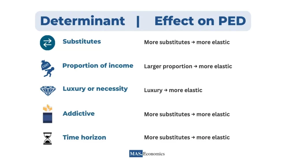
Availability of substitutes. The more close substitutes a good has, the more elastic its demand. A consumer who finds her preferred soda brand more expensive can switch to another at near-zero cost. A patient who needs a specific medication with no chemical equivalent cannot. The first market is elastic; the second is inelastic. Substitutability is the single most important determinant in most empirical studies.

Necessity versus luxury. Necessities (basic food, electricity, insulin, fuel for daily commuting) tend to have inelastic demand because consumers continue buying even when prices rise. Luxuries (premium watches, designer goods, second homes) have elastic demand because purchases can be postponed or skipped entirely. The distinction is not absolute. Whether a car is a necessity or a luxury depends on whether public transport is a viable alternative, which is why income elasticity often runs alongside price elasticity in empirical work.

Share of the budget. A good that consumes a large share of household income tends to have more elastic demand because the same percentage price change has a larger absolute effect on the budget. Salt has inelastic demand partly because doubling its price leaves household finances unaffected. Housing has more elastic demand at the margin because the absolute amounts are large enough to force lifestyle adjustments.

Time horizon. Demand becomes more elastic over time. After the oil shocks of the 1970s, short-run estimates of gasoline price elasticity were around −0.1, meaning a 10 percent price increase cut consumption by only 1 percent. Long-run estimates, after consumers had time to switch to more fuel-efficient vehicles, move closer to −0.6 or −0.8. The same good can carry very different elasticities depending on which horizon is being measured.

Addictiveness and habit formation. Goods that generate physical or psychological dependence (tobacco, caffeine, and gambling) show particularly inelastic demand in the short run, which is precisely why governments tax them. Smokers continue purchasing cigarettes even when prices double, although long-run elasticity is higher as some users quit and new initiates decline.

Applications of Price Elasticity of Demand

Tax policy. A government raising revenue prefers to tax goods with inelastic demand because consumers continue purchasing despite higher prices. This is why excise duties on fuel, tobacco, and alcohol are revenue workhorses in nearly every fiscal system. A government trying to discourage consumption of a particular good (sugar-sweetened beverages, for example) achieves more behavioral change by taxing a good with more elastic demand, though the revenue may decline as quantity contracts.

Firm pricing. A firm facing elastic demand cannot easily raise prices because consumers will switch to alternatives or postpone purchases. A firm facing inelastic demand can raise prices and watch total revenue rise. The pharmaceutical industry has built a business model around this dynamic, securing patent protection precisely to convert what would otherwise be elastic demand into inelastic demand by removing close substitutes.

Tax incidence. The party that bears more of a tax burden is the one with the more inelastic side of the market. When demand is inelastic relative to supply, consumers pay most of the tax. When supply is inelastic relative to demand, producers absorb most of it. The split depends on the relative magnitudes of PED and PES, which is one of the few applied predictions in microeconomics where the math actually has to balance.

Price Elasticity of Supply

Price elasticity of supply (PES) measures how the quantity supplied of a good responds to a change in its price. The formula is structurally identical to PED but applied to producers:

PRICE ELASTICITY OF SUPPLY

PES is typically positive because price and quantity supplied move in the same direction.

The categorization mirrors PED. Elastic supply carries PES greater than one, meaning producers can ramp output up or down quickly when prices move. Inelastic supply carries PES below one, meaning output barely responds even to large price changes. Unit elastic supply sits at one. Two extreme cases bookend the range: perfectly inelastic supply at PES equal to zero (the quantity is fixed regardless of price, as with a rare artwork already produced), and perfectly elastic supply at PES approaching infinity (suppliers will provide any quantity at the prevailing price).

The image below contrasts elastic and inelastic supply curves.

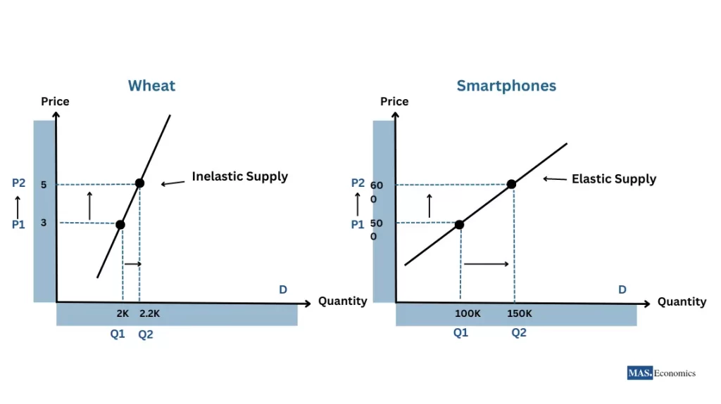
The steeper supply curve represents a crop like wheat, where farmers cannot expand the harvest mid-season regardless of how high prices climb. The flatter supply curve represents a manufactured good like smartphones, where factories can add shifts, draw on inventory, or expand production lines relatively quickly when prices rise.

Consider two worked examples. A poor harvest pushes wheat prices from $5 to $7 per bushel, a 40 percent increase. Global supply rises from 2,000 to 2,200 bushels, a 10 percent increase. The PES is:

A PES of 0.25 indicates a highly inelastic supply. Farmers are constrained by growing seasons, land availability, and seed supplies. In the short run, they cannot meaningfully expand output even when prices spike. Over a longer horizon, more land may be brought into wheat production, and the elasticity rises.

Now consider a different sector. A surge in demand pushes smartphone prices from $500 to $600, a 20 percent increase. Manufacturers respond by raising output from 100,000 to 150,000 units, a 50 percent increase. The PES is:

A PES of 2.5 indicates elastic supply. Factories can add shifts, accelerate component orders, and tap inventory. The contrast between 0.25 for wheat and 2.5 for smartphones illustrates the central insight: supply elasticity depends primarily on how quickly producers can adjust their production process.

Determinants of Price Elasticity of Supply

Spare capacity. A firm running below full capacity can ramp output quickly when prices rise. A firm already running flat out cannot. Industries with cyclical demand often carry deliberate spare capacity precisely because it makes supply elastic during peaks, allowing firms to capture revenue from temporary price spikes.

Time horizon. In the short run, at least one factor of production is fixed (factory space, equipment, land area). Supply is inelastic. In the long run, firms can expand capacity, new entrants can join the market, and supply becomes more elastic. The difference between short-run and long-run supply elasticity is often a factor of three to five, which is why supply shocks have larger price effects in the immediate term and smaller ones over a multi-year horizon.

Availability of inputs. Production requires raw materials, components, skilled labor, and energy. If any one input is scarce or specialized, supply cannot expand even when prices rise. The semiconductor shortage of 2021 to 2022 made automobile supply highly inelastic because manufacturers could not source chips at any reasonable price, regardless of how much consumers were willing to pay for finished vehicles.

Specialization. A factory designed for one product cannot be repurposed quickly. Highly specialized production (custom industrial equipment, certain pharmaceuticals) carries an inelastic short-run supply. More flexible production lines, such as those used in textile or food processing, allow for faster output changes.

Storability and inventory. Goods that store well allow producers to manage supply by drawing from or adding to inventory. Non-perishable commodities (grains, metals, oil) carry a more elastic short-run supply than perishables (fresh produce, dairy) because inventory smooths the response to price changes.

Applications of Price Elasticity of Supply

Capacity planning. Firms in industries with inelastic supply can capture temporary price spikes because competitors cannot quickly expand output. Firms in elastic-supply industries face the opposite dynamic: any price advantage is competed away as rivals add capacity. The two business models call for different pricing strategies and different attitudes toward inventory.

Agricultural policy. Governments setting minimum support prices for crops are betting on inelastic short-run supply (farmers cannot easily increase plantings within one season) and more elastic long-run supply (farmers will respond over multiple years). Misjudging the elasticity has produced repeated cycles of glut and shortage in agricultural markets, from the European Common Agricultural Policy to India’s wheat and rice procurement system.

Resource extraction. Oil supply is famously inelastic in the short run because bringing new wells online takes years. This is the mechanism behind the explosive oil price spikes of 1973, 1979, 2008, and 2022. Long-run supply is much more elastic as exploration, development, and unconventional sources respond to sustained high prices, which is also why every oil price spike has eventually unwound.

The Time Horizon Matters as Much as the Number

One pattern unites PED and PES: both elasticities increase with time. Consumers and producers both have more options when they have more time to act. A consumer facing a sudden gasoline price spike has few short-run alternatives but can switch to public transit, carpool, or buy a fuel-efficient car over a longer horizon. A producer facing a sudden price spike cannot expand factories overnight, but can do so within a year or two.

Empirical work distinguishes routinely between immediate response (one month or one quarter), short run (one year), and long run (three to five years or longer). The distinction matters because policy decisions made on short-run elasticity estimates often underestimate how much markets eventually adjust. A fuel tax that looks like a pure revenue raiser based on short-run elasticity may, over five years, generate significantly more behavioral change as consumers transition to alternatives.

Explains

Conclusion

The price elasticity of demand and supply turns directional facts about markets into quantitative ones. Knowing that demand falls when price rises is rarely enough. Whether the fall is one percent or ten percent determines whether a tax raises revenue or destroys it, whether a price cut boosts profits or shrinks them, and whether a supply disruption causes a mild inconvenience or an economic crisis. The two elasticities are the workhorses of applied price theory, and their values are estimated and re-estimated for every commodity and service of policy interest.

Three things matter when reading any elasticity estimate. The first is the horizon: short-run and long-run values can differ by orders of magnitude. The second is the substitution environment: an elasticity estimated in one market with one set of alternatives may not transfer to another market or another period. The third is the structural framing: tax incidence, revenue projections, and capacity decisions all depend on the joint behavior of PED and PES, not on either one in isolation. The numbers are useful, but they are most useful when paired with an understanding of the institutional setting that produced them.

Frequently Asked Questions

Thanks for reading! If you found this helpful, share it with friends and spread the knowledge. Happy learning with MASEconomics