IS-LM-BP Model: Open Economy Equilibrium Diagram

When a country opens its capital account, the central bank loses the comfort of treating interest rates as a purely domestic instrument. A rate set too far above world levels pulls in foreign capital and pushes the currency or reserves; a rate set too far below sends capital out. The IS-LM-BP model is the diagram economists use to make that tension visible. It takes the closed-economy goods-and-money framework and adds a third schedule for the external balance, so that goods market equilibrium, money market equilibrium, and balance-of-payments equilibrium all have to hold at the same interest rate and the same level of output.

The model is the graphical core of the open-economy macroeconomics developed by Robert Mundell and J. Marcus Fleming in the early 1960s. It is the same machinery that sits behind the Mundell-Fleming model, presented here as a single equilibrium picture rather than a set of policy experiments. Reading that picture correctly is the prerequisite for everything that follows: why fiscal policy behaves one way under fixed exchange rates and another way under floating rates, and why the slope of one curve decides whether monetary policy moves output at all.

Three Markets, One Interest Rate

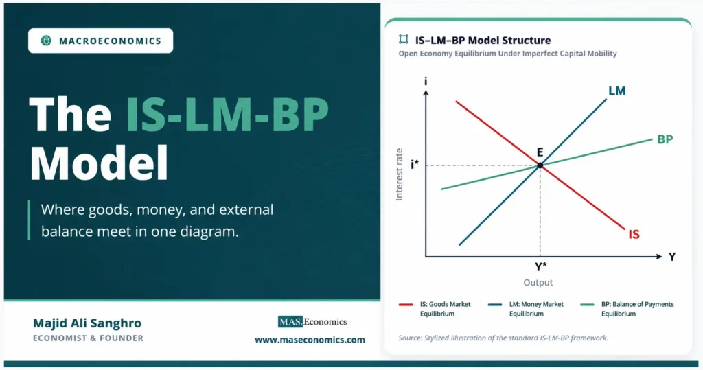
The diagram lives in a plane with real output \(Y\) on the horizontal axis and the domestic nominal interest rate \(i\) on the vertical axis. Every point in that plane describes a combination of output and interest rate. The three schedules each pick out the combinations consistent with equilibrium in one market, and the economy as a whole is in equilibrium only where all three conditions are satisfied together.

The first schedule is the IS curve, which traces goods market equilibrium. It comes directly from the IS-LM framework used for closed economies, with one adjustment: in an open economy, planned spending includes net exports, so the IS relation depends on the real exchange rate as well as on income and the interest rate. Goods market equilibrium requires that output equals planned expenditure.

Goods Market (IS)

Net exports NX depend on home income Y, foreign income Y*, and the real exchange rate e. Investment I falls as the interest rate i rises.

Because higher output raises imports and a higher interest rate cuts investment, the combinations that keep the goods market in balance slope downward in the \(Y\)-\(i\) plane: a rise in the interest rate must be matched by lower output to keep spending equal to production. That downward slope is the IS curve.

The second schedule is the LM curve, which traces money market equilibrium. Real money supply is set by the central bank and the price level; real money demand rises with output (more transactions) and falls with the interest rate (a higher opportunity cost of holding money).

Money Market (LM)

Real money demand L increases in output Y and decreases in the interest rate i. With M and P fixed in the short run, the relation defines an upward-sloping schedule.

Holding the real money stock fixed, a rise in output raises money demand, which can only be reconciled with a fixed supply if the interest rate rises to choke demand back. The combinations that keep the money market in balance therefore slope upward. That upward slope is the LM curve.

Where IS and LM cross, the goods and money markets clear together. In a closed economy, the story ends there. In an open economy it does not, because that internal equilibrium says nothing about whether the country’s external accounts balance. The third schedule supplies the missing condition.

BP Curve and Slope Interpretation

The balance-of-payments schedule, the BP curve, traces the combinations of output and interest rate at which the external accounts are in equilibrium, meaning the current account and the capital account sum to zero. It rests on the accounting identity behind the balance of payments: a deficit on the current account has to be financed by a surplus on the capital and financial account, and vice versa.

Two forces pull in opposite directions along the BP curve. Higher domestic output raises imports, which worsens the current account. A higher domestic interest rate attracts foreign capital, which improves the capital account. For the overall balance to stay at zero, the two effects must offset. A rise in output that drags the current account into deficit has to be paired with a higher interest rate that pulls in enough capital to finance it. That requirement gives the BP curve its upward slope.

External Balance (BP)

The capital account KA rises with the gap between the domestic and foreign interest rate (i − i*). External balance requires the current and capital accounts to sum to zero.

The slope of the BP curve is not a cosmetic detail. It encodes the degree of capital mobility, and it is the single feature of the diagram that determines how powerful monetary and fiscal policy will be. The intuition runs through how strongly capital flows respond to the interest-rate differential \(i – i^{*}\).

When capital is perfectly mobile, the smallest interest-rate gap triggers unlimited capital flows. No domestic interest rate can persist above or below the world rate \(i^{*}\), so the BP curve is horizontal at \(i = i^{*}\). When capital is perfectly immobile, the capital account cannot respond at all, external balance depends entirely on the current account, and only one level of output is consistent with it; the BP curve is vertical. The realistic case of imperfect mobility sits between these, producing an upward-sloping BP curve whose steepness measures how reluctantly capital crosses borders.

Equilibrium Where All Three Cross

Open-economy equilibrium is the point where the IS, LM, and BP curves intersect simultaneously. At that point the goods market clears, the money market clears, and the balance of payments is in equilibrium, all at one interest rate and one level of output. The diagram below shows the standard case of imperfect capital mobility, where the BP curve slopes upward and all three schedules meet at a single point.

The economy will not sit anywhere except point E. To see why, consider a point on the IS-LM intersection that does not lie on the BP curve. Suppose internal equilibrium occurs at an interest rate below the level the BP curve requires for that output. The interest-rate gap is too small to attract the capital needed to finance the trade deficit, so the balance of payments runs a deficit. Under fixed exchange rates, the central bank sells reserves to defend the parity, the money supply contracts, and the LM curve shifts left until it passes through the BP curve. Under floating exchange rates, the currency depreciates, net exports improve, and the IS and BP curves shift until they meet the LM intersection. Either way, the adjustment continues until all three curves cross.

This is the deepest point the diagram teaches. The internal balance described by IS-LM is not the end of the story in an open economy. External pressure forces an adjustment that the closed-economy model never anticipates, and the channel of that adjustment, reserves and the money supply or the exchange rate, depends entirely on the exchange-rate regime.

Interacting Slopes of IS, LM, BP

The relative slopes of the LM and BP curves carry most of the model’s predictive content. Both slope upward, but their steepness reflects different economics. The LM slope reflects the interest sensitivity of money demand. The BP slope reflects the degree of capital mobility. Whether the BP curve is flatter or steeper than the LM curve changes how a policy shift plays out, which is why the comparative-statics experiments treated in the rest of this cluster always begin by fixing the slope of BP relative to LM.

Table 1. Capital Mobility and the Shape of the BP Curve

Capital mobility	BP curve shape	What it implies
Perfect	Horizontal at \(i = i^{*}\)	Domestic rate cannot deviate from the world rate
High but imperfect	Upward sloping, flatter than LM	Capital responds strongly to small rate gaps
Low but imperfect	Upward sloping, steeper than LM	Capital responds weakly; current account dominates
Zero	Vertical	Only one output level clears the external account
Source: MASEconomics editorial synthesis of the standard Mundell-Fleming framework.

The horizontal and vertical cases are not just textbook curiosities. The horizontal BP curve is the assumption behind the sharpest Mundell-Fleming results, the ones that say monetary policy is powerless under fixed rates and fiscal policy is powerless under floating rates. Relaxing perfect mobility to an upward-sloping BP curve softens those conclusions, because the domestic interest rate is then free to move away from the world rate, and the size of that freedom is exactly what the BP slope measures.

Assumptions and Limitations of the Diagram

The IS-LM-BP diagram is a short-run model. Prices are fixed, so the real money stock moves only when the central bank changes the nominal money supply or, under fixed rates, when reserve flows force the change. Expectations about the exchange rate are held constant, which is why the model cannot say anything about exchange-rate dynamics on its own; the Dornbusch overshooting model was built precisely to add the expectations channel the static diagram leaves out.

The model also treats the world interest rate \(i^{*}\) and foreign output \(Y^{*}\) as given, which is reasonable for a small economy but strained for a large one whose policy moves world markets. And it says nothing about the long-run constraint that a country cannot run capital-account surpluses forever to finance trade deficits, the solvency question that the monetary approach to the balance of payments takes as its starting point.

These limits are features, not flaws. By freezing prices and expectations, the diagram isolates the one thing it is built to show: how the goods, money, and external markets reconcile through the interest rate and output, and how the exchange-rate regime decides which variable does the adjusting. That isolation is what makes the comparative-statics experiments in the rest of this cluster legible. Once the single equilibrium is understood, shifting any one curve and tracing the economy back to a new triple intersection becomes a disciplined exercise rather than a guess.

Conclusion

The IS-LM-BP model earns its place by adding one curve to a familiar diagram and, with it, an entire dimension of macroeconomic constraint. Goods market equilibrium gives the downward‑sloping IS curve, money market equilibrium gives the upward‑sloping LM curve, and external balance gives the BP curve whose slope encodes how freely capital crosses borders. Equilibrium is the single point where all three cross, and the economy is pushed toward that point by reserve flows under fixed exchange rates or by exchange‑rate movements under floating rates.

The decisive lesson is that internal balance is not enough in an open economy. A combination of output and interest rate can clear the goods and money markets and still leave the balance of payments in deficit or surplus, and the resulting pressure forces an adjustment whose channel depends on the exchange‑rate regime. The slope of the BP curve relative to the LM curve then governs how strongly monetary and fiscal policy can move output at all.

That structure is why the diagram is the foundation for the comparative‑statics results that follow. Fixed exchange rates, floating exchange rates, and the full range of capital‑mobility cases are all read off the same three‑curve picture by shifting one schedule and locating the new triple intersection. The equilibrium diagram is the grammar; the policy experiments are the sentences written in it.

Frequently Asked Questions

Thanks for reading! If you found this helpful, share it with friends and spread the knowledge. Happy learning with MASEconomics