A researcher has thirty annual observations, a theory that says two variables move together in the long run, and a unit root test that says one series is clearly non-stationary, another is clearly stationary, and a third is somewhere on the boundary. The standard cointegration methods refuse the job: Engle-Granger and Johansen both require every variable to be integrated of order one, and pre-testing to establish that is exactly the step the data will not settle. The ARDL bounds test was built for this situation. It tests for a long-run relationship without requiring the researcher to classify each series first, it works on short samples, and it delivers the long-run coefficients and the speed of adjustment from a single equation. That combination is why it dominates applied macroeconomic work in exactly the settings where data is short and mixed.
The Problem It Solves
Cointegration means that variables which individually wander can move together in the long run, so that some combination of them is stationary. Testing for it conventionally begins with unit root tests on every series, and that first step carries the whole procedure. Unit root tests have low power in short samples, which is our article on stationarity put uncomfortably: the augmented Dickey-Fuller test often fails to reject a unit root in a series that is stationary, and a structural break makes that failure more likely still. Every subsequent step inherits whatever the classification got wrong.
The two classical approaches make that inheritance total. The Engle-Granger method, described in our article on cointegration and Engle-Granger, regresses the levels and tests the residuals for stationarity, which requires all variables to be integrated of the same order and handles only one long-run relationship. The Johansen procedure, built inside the vector framework our article on VAR and VECM models covers, can find several relationships at once but assumes every variable is integrated of order one and needs a longer sample to estimate its system reliably.
The autoregressive distributed lag approach of Pesaran, Shin and Smith removes the pre-classification requirement. Its bounds test is valid whether the regressors are stationary, integrated of order one, or a mixture of the two, so the awkward series that the unit root test could not settle no longer blocks the analysis. It estimates a single equation rather than a system, which is why it performs comparatively well on the sample sizes that macroeconomic work on individual countries usually has.
One Equation, and the Test Inside It
The method starts from an unrestricted error correction form. Regress the change in the dependent variable on its own lagged changes, on current and lagged changes of the regressors, and, above all, on the lagged levels of everything.
The lagged level terms are where the long run lives. If no long-run relationship exists, those levels carry no information about the change and their coefficients should jointly be zero. The bounds test is precisely that joint restriction.
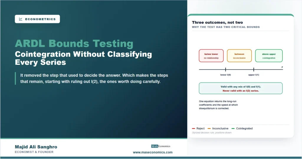
What makes the test unusual is not the statistic, which is an ordinary F test of a joint restriction of the kind our article on hypothesis testing describes. It is the critical values. Because the regressors may be stationary or integrated of order one and the researcher is not required to say which, the distribution of the statistic is not a single one but lies between two. Pesaran, Shin and Smith tabulated both: a lower bound computed as if every regressor were stationary, and an upper bound computed as if every regressor were integrated of order one. The comparison then has three possible outcomes rather than two.
An inconclusive result is a genuine outcome and not a licence to pick the convenient bound. The disciplined responses are to consult the t statistic on the lagged dependent variable in levels, which Pesaran and colleagues tabulate alongside the F bounds, to use critical values computed for small samples rather than the asymptotic ones when the sample is short, since the asymptotic values reject too rarely in samples of thirty or forty observations, and to say plainly in the write-up that the test did not resolve. Reporting the F statistic and the two bounds lets a reader see that for themselves, which is why all three numbers belong in the table.
The Long Run and the Speed of Return to It
Once cointegration is established, the same equation yields both halves of the answer. The long-run coefficients are recovered from the lagged level terms: the long-run effect of the regressor on the dependent variable is the negative of its level coefficient divided by the level coefficient on the dependent variable. That single line is what the whole exercise was for, and it is the number a theory usually predicts.
The short run is then re-estimated in error correction form, with the deviation from the long-run relationship entering as one term.
The coefficient on the error correction term is the most informative single number the method produces, and it has to satisfy two conditions to be believed. It must be negative, because a positive coefficient means deviations grow rather than close, which contradicts the cointegration the test just accepted. And it must be statistically significant, since an insignificant term means nothing is pulling the system back. Its magnitude is then read directly: a coefficient of minus zero point four means roughly forty percent of the previous period’s disequilibrium is corrected within one period, so adjustment takes about two and a half periods to work through. On annual data that is a slow but plausible economy; a coefficient close to minus one implies almost complete adjustment within a year, which is worth questioning on annual macroeconomic data; and a coefficient below minus one implies overshooting and oscillation, which usually indicates a misspecified model rather than a discovery.
| Feature | Engle-Granger | Johansen | ARDL bounds |
|---|---|---|---|
| Integration order required | All I(1) | All I(1) | Any mix of I(0) and I(1); never I(2) |
| Pre-testing for unit roots | Essential, and decisive | Essential, and decisive | Only to rule out I(2) |
| Long-run relationships found | One | Several, and it counts them | One |
| Sample size needed | Moderate | Large, since a system is estimated | Works on short samples |
| Short and long run together | Two steps | Yes, within the system | Yes, from one equation |
| Endogenous regressors | Assumed away | Handled by construction | Handled by lag structure, with limits |

|
|||
The Five Rules That Get Broken
The method’s accessibility is also how it is misused, and the same handful of errors recur in submitted work.
The first and most serious is skipping the check for second-order integration. ARDL frees the researcher from classifying series as stationary or first-order integrated, and it does not free them from ruling out I(2). The bounds critical values are simply not valid when a variable needs differencing twice, so a unit root test still has to be run, not to classify every series but to establish that none is I(2). The second is lag selection treated as an afterthought. Lags are chosen by an information criterion, usually Akaike or Schwarz, and the two disagree in short samples, with Akaike choosing longer lags and Schwarz more parsimonious ones; the choice changes the test statistic, so the criterion used and the maximum lag allowed both belong in the write-up, a decision our article on choosing an econometric model treats as substantive rather than clerical.
The third is ignoring parameter stability. The bounds procedure assumes the relationship holds across the sample, and macroeconomic series covering several decades routinely contain the regime shifts our article on structural breaks describes. The CUSUM and CUSUM of squares plots are the conventional check and they cost nothing to produce. The fourth is publishing the long-run coefficients without the diagnostics. An equation with autocorrelated residuals has invalid standard errors on those coefficients, so the tests in our article on autocorrelation are part of the result rather than an appendix, alongside the usual checks on functional form and normality.
The fifth is conceptual. A bounds test that rejects tells you a stable long-run relationship exists among the variables in the equation; it does not tell you which variable drives which. Direction comes from theory or from a design that identifies it, and the single-equation structure quietly assumes the regressors are weakly exogenous. Where that assumption is doubtful and the sample allows it, the system approach in our article on vector autoregression is the more honest tool. ARDL is a way of testing a relationship the researcher has reasons to expect, not a way of discovering one.
MASEconomics Explains
3 econometric concepts behind the bounds test
These concepts are explored in depth across our educational articles library.
Conclusion
The ARDL bounds test earns its place by removing a step that used to decide everything. Because it is valid whether the regressors are stationary, first-order integrated or mixed, the researcher no longer has to classify each series correctly before beginning, which matters most in exactly the short macroeconomic samples where unit root tests are least reliable. One unrestricted error correction equation carries the whole procedure: the joint test on the lagged levels asks whether a long-run relationship exists, the level coefficients deliver it if it does, and the error correction term measures how quickly the system returns to it.
The discipline is in the details that are easy to skip. Confirm no variable is integrated of order two, because the critical values assume it. Report the F statistic with both bounds, and call an inconclusive result inconclusive. State the lag criterion and the maximum lag, since the statistic depends on them. Show the stability plots and the residual diagnostics, because the long-run coefficients inherit whatever is wrong with the equation. And remember what a rejection establishes: that these variables share a stable long-run relationship, not which one moves first. The method tests a relationship worth expecting; it does not supply the reason for expecting it.
Frequently Asked Questions
What is the ARDL bounds test used for?
To test whether a long-run relationship exists among variables when their orders of integration are mixed or uncertain. It is valid with stationary regressors, first-order integrated regressors, or a combination, so the researcher does not need to classify each series correctly beforehand. It also returns the long-run coefficients and the speed of adjustment from the same equation.
Why does the bounds test have two critical values?
Because the distribution of the statistic depends on whether the regressors are stationary or integrated, and the method deliberately avoids requiring that to be settled. The lower bound is computed as if all regressors were stationary, the upper as if all were first-order integrated. Above the upper bound a long-run relationship is accepted, below the lower it is rejected, and between them the test genuinely cannot say.
Can ARDL be used with I(2) variables?
No. The tabulated critical values assume no variable requires differencing more than once, so a series integrated of order two invalidates the test. This is why unit root testing is still necessary under ARDL: not to classify every series as stationary or first-order integrated, but to establish that none is I(2). Skipping that check is the most common misuse of the method.
What does the error correction term coefficient mean?
It is the share of the previous period’s deviation from the long-run relationship that is corrected in the current period. It must be negative and statistically significant for the model to be coherent. A value of minus zero point four means about forty percent of the gap closes each period; a value below minus one implies overshooting and usually indicates misspecification rather than a finding.
What should be done when the bounds test is inconclusive?
Report it as inconclusive, and then use the supporting evidence rather than choosing the convenient bound. The t statistic on the lagged dependent variable in levels has its own tabulated bounds and can be informative. Critical values computed for small samples are more appropriate than asymptotic ones when the sample runs to thirty or forty observations. Extending the sample or reconsidering the lag length are the other honest options.
When is Johansen better than ARDL?
When the sample is long enough to estimate a system, when all variables are first-order integrated, and above all when several long-run relationships may exist, since Johansen tests how many there are while ARDL assumes one. Johansen also handles endogeneity by construction, whereas the single-equation ARDL assumes the regressors are weakly exogenous.
Thanks for reading! The method removed the step that used to decide the answer, which makes the remaining steps the ones worth doing carefully. Happy learning with MASEconomics