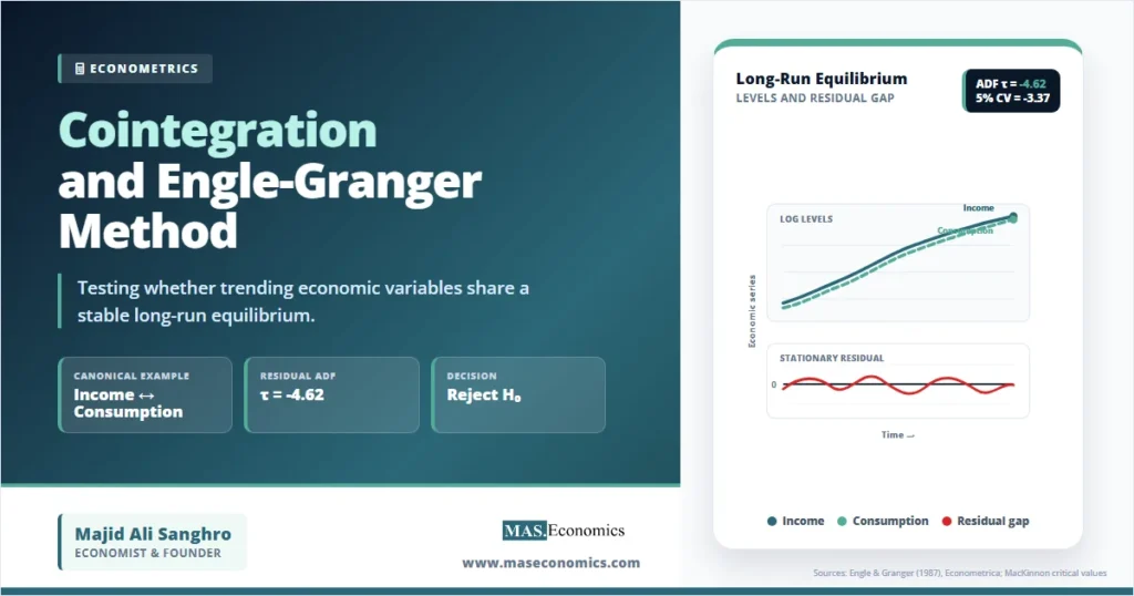
A regression between consumption and income can look excellent while being statistically false. Both series may trend upward, the fitted line may produce a high \(R^2\), and the t-statistics may look convincing. The statistical sin is spurious regression: non-stationary variables can appear related because they share stochastic trends, not because they obey a stable economic law. Cointegration and Engle-Granger Method solve this problem by asking whether the regression residual is stationary. If the residual is stationary, the variables drift in the short run but remain tied by a long-run equilibrium.
Cointegration matters because many macroeconomic variables are persistent. Income, consumption, prices, money balances, exports, imports, exchange rates, and public debt often behave like integrated processes. Regressing one trending variable on another without checking the time-series structure can turn noise into a policy story. The Engle-Granger method gives applied economists a disciplined way to separate a genuine long-run relation from a misleading trend correlation.
The method was formalised by Robert Engle and Clive Granger in their 1987 Econometrica paper, “Co-integration and Error Correction: Representation, Estimation, and Testing”. Their key insight was not only a test. It was a representation theorem: when integrated variables are cointegrated, they can be represented through an error-correction model. That theorem connects long-run equilibrium to short-run adjustment, which is why cointegration became central to applied macroeconometrics.
Stochastic Trends That Refuse to Disappear
Let \(y_t\) and \(x_t\) be two economic time series. If each series is integrated of order one, written \(I(1)\), each becomes stationary after first differencing:
The problem is that a regression in levels can still look persuasive even when the variables have no meaningful relationship. Granger and Newbold’s classic work on spurious regressions in econometrics showed why high fit and statistically meaningful coefficients can arise when unrelated non-stationary series are regressed on each other. In such cases, conventional OLS inference breaks because the assumptions behind the usual t and F distributions fail.
Cointegration changes the interpretation. The two variables may each contain a stochastic trend, but a particular linear combination may remove that common stochastic trend. For a bivariate relationship, cointegration exists if there is a coefficient \(\beta\) such that:
Here \(u_t\) is the equilibrium error. If \(u_t\) is stationary, deviations from the long-run relationship are temporary. The series can wander, but its distance from the equilibrium line does not explode. This is the mathematical distinction between a valid long-run regression and a spurious regression.
The Long-Run Equation and Residual Test
The Engle-Granger method begins with the long-run cointegrating regression:
The null and alternative hypotheses are written in terms of the residual \(u_t\):
The residual is not observed directly. It is estimated from OLS:
The second step tests whether \(\hat{u}_t\) has a unit root. The usual residual-based ADF regression is:
The null hypothesis is \(\rho = 0\), meaning the residual has a unit root. The alternative is \(\rho < 0\), meaning the residual is stationary. The test statistic is:
The decision rule differs from the standard ADF test because the residual \(\hat{u}_t\) is generated from a prior estimated regression. Standard Dickey-Fuller critical values are not valid. Engle-Granger residual tests require cointegration-specific critical values, such as those tabulated and refined by MacKinnon in Critical Values for Cointegration Tests. More negative values of \(\tau_{EG}\) provide stronger evidence against the null of no cointegration.
The method can be extended to include deterministic components. A long-run regression may include an intercept only, an intercept and trend, or other deterministic terms. The chosen deterministic structure changes the relevant critical values. A trend in the cointegrating equation is not a harmless decoration. It changes the null distribution of the test statistic.
If cointegration is found, the next equation is an error-correction model:
The parameter \(\lambda\) is the speed of adjustment. A negative \(\lambda\) means that when \(y_t\) is above its long-run equilibrium relative to \(x_t\), future changes in \(y_t\) tend to pull the system back. Engle and Granger’s representation theorem links cointegration and error correction: a cointegrated system has an error-correction representation, and an error-correction model implies cointegration under the relevant conditions.
For readers building the wider econometrics cluster, the Engle-Granger method links naturally to what econometrics is, structural breaks in time series analysis, distributed lag models, and multivariate time series models. Cointegration is where time-series persistence, equilibrium theory, and dynamic adjustment meet.
How the Two-Step Test Computes Evidence
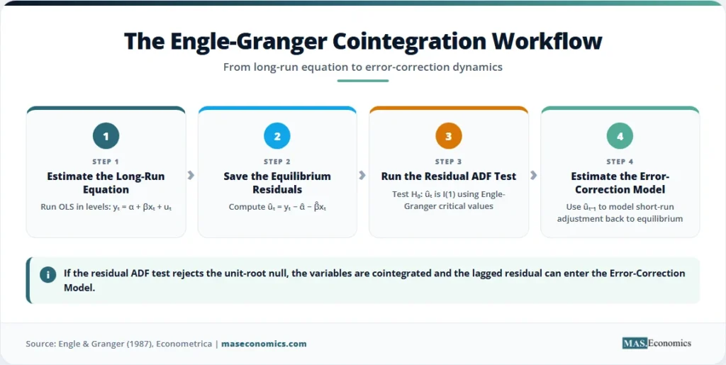
The first computational step is the long-run OLS projection. Suppose the variable \(y_t\) is log consumption and \(x_t\) is log disposable income. OLS chooses \(\hat{\alpha}\) and \(\hat{\beta}\) to minimise the sum of squared equilibrium errors:
This regression is not interpreted through ordinary t-statistics at this stage. The key object is the residual series \(\hat{u}_t\). If consumption and income share a long-run equilibrium, the residual should behave like a stationary gap. It should fluctuate around zero rather than drifting permanently away from it.
The second step estimates the residual ADF equation. Lagged differences \(\Delta \hat{u}_{t-j}\) are included to absorb short-run serial correlation in residual changes. The lag length \(p\) can be selected using an information criterion such as AIC or BIC, or by checking whether the remaining residuals are approximately serially uncorrelated. The test focuses on \(\hat{\rho}\), not on the short-run lag coefficients.
The third step compares \(\tau_{EG}\) with Engle-Granger critical values. If the statistic is more negative than the critical value, the unit-root null for the residual is rejected. The conclusion is not that \(y_t\) and \(x_t\) are individually stationary. The conclusion is that their estimated long-run residual is stationary, so the two variables are cointegrated.
The fourth step estimates an error-correction model. At this point, the long-run residual becomes an explanatory variable in the short-run equation. The coefficient on \(\hat{u}_{t-1}\) tells how quickly disequilibrium closes. A value of \(-0.30\), for example, means about 30 percent of last period’s equilibrium gap is corrected in the current period, conditional on the included short-run changes.
Consumption and Income in Equilibrium
Consider a stylised annual dataset with 80 observations. Log consumption and log disposable income are both \(I(1)\). The canonical economic claim is simple: households spend a stable share of long-run income, but short-run consumption can deviate from that path because of credit conditions, expectations, temporary tax changes, or measurement noise.
| Equation / Test | Estimate | Standard Error | Test Statistic | Decision |
|---|---|---|---|---|
| Long-run intercept \(\hat{\alpha}\) | 0.400*** | (0.080) | 5.00 | Long-run constant retained |
| Long-run income elasticity \(\hat{\beta}\) | 0.920*** | (0.030) | 30.67 | Economic magnitude: near proportional |
| Residual ADF coefficient \(\hat{\rho}\) | -0.380*** | (0.082) | -4.62 | Reject \(H_0\): no cointegration |
| 5% Engle-Granger critical value | -3.37 | n/a | n/a | \(-4.62 < -3.37\) |
| Error-correction speed \(\hat{\lambda}\) | -0.310** | (0.120) | -2.58 | 31% of gap closes per year |
| Short-run income growth \(\hat{\theta}\) | 0.450** | (0.190) | 2.37 | Positive short-run pass-through |
| Observations | 80 | Annual stylised sample | ||
| Residual ADF lags | 1 | Selected by BIC | ||
| Cointegrating regression \(R^2\) | 0.96 | Not used as proof of validity | ||

|
||||
The long-run equation implied by the table is:
The estimated income elasticity is 0.920. A 1 percent increase in long-run disposable income is associated with a 0.92 percent increase in long-run consumption. That coefficient is economically plausible because consumption rises almost proportionally with income, but not mechanically one-for-one.
The cointegration decision comes from the residual ADF statistic, not from the high \(R^2\). The estimated test statistic is \(-4.62\). The 5 percent Engle-Granger critical value for this stylised setup is \(-3.37\). Since \(-4.62\) is more negative than \(-3.37\), the null hypothesis of no cointegration is rejected. The residual from the long-run consumption-income equation is stationary.
The error-correction coefficient is \(-0.310\). If consumption is above its long-run level relative to income, the negative coefficient predicts slower consumption growth in the next period. If consumption is below equilibrium, the same coefficient predicts faster adjustment upward. In this stylised example, about 31 percent of the disequilibrium gap closes per year.
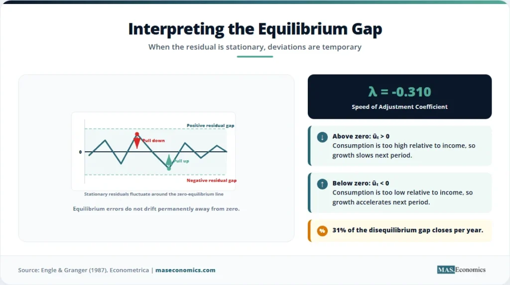
The visual logic is direct. Log income and log consumption trend upward together, so a levels regression would be suspicious without further testing. The residual gap, however, oscillates around zero. That stationary gap is the empirical signature of cointegration. The series may move apart temporarily, but they do not drift apart indefinitely.
Where Engle-Granger Breaks Down
The Engle-Granger method is powerful because it is simple. That same simplicity creates limits. The first limit is the single-equation structure. In a bivariate setting, there can be only one cointegrating vector. In larger systems, there may be multiple long-run relationships. The Engle-Granger approach cannot estimate the rank of the cointegration space in the way system methods such as Johansen testing can.
The second limit is normalisation. Regressing \(y_t\) on \(x_t\) can produce a different residual from regressing \(x_t\) on \(y_t\). In finite samples, the Engle-Granger result may depend on which variable is placed on the left-hand side. That is not a small detail when economic theory does not clearly define the dependent variable.
The third limit is low power. Residual-based tests may fail to reject the null of no cointegration even when a long-run relationship exists, especially in short samples or when adjustment is slow. Macroeconomic datasets often contain only a few decades of annual observations. A weak test result may reflect limited information rather than the absence of equilibrium.
The fourth limit is structural instability. Cointegration assumes a stable long-run relationship over the sample. A policy regime change, financial liberalisation, pandemic shock, exchange-rate realignment, or tax reform can alter the intercept, slope, or adjustment speed. When the cointegrating vector changes, a residual test applied to the full sample can mislead. This connects cointegration directly to structural break analysis.
The fifth limit is the order of integration. Engle-Granger is designed for variables that are integrated of the same order, most commonly \(I(1)\). Mixing \(I(0)\), \(I(1)\), and \(I(2)\) variables without care can produce invalid inference. Testing the integration properties of each variable is therefore not optional. It is part of the identification of the time-series environment.
Residual-based cointegration tests have also been extended and scrutinised in later econometric work. Phillips and Ouliaris developed an asymptotic theory for residual-based tests, including links between ADF-type and \(Z_t\)-type statistics. Federal Reserve research has also examined residual-based cointegration tests when variables are near unit root rather than exact unit-root processes, showing how nuisance parameters can complicate inference in borderline cases.
Why Economists Use It in Policy Models
Cointegration is common in economics because theory often predicts long-run equilibrium, while data show short-run disequilibrium. Consumption and income, money demand and interest rates, imports and domestic absorption, exports and foreign income, spot and futures prices, exchange rates and fundamentals, government revenue and expenditure, and prices across linked markets all fit this pattern. The short run is noisy. The long run is disciplined by budget constraints, arbitrage, accounting identities, or behavioural adjustment.
In macroeconomics, cointegration helps model money demand. A central bank may believe real money balances depend on real income and interest rates in the long run. If the variables are non-stationary, a levels regression can be invalid unless the residuals are stationary. A cointegrated money-demand equation allows the central bank to estimate both the long-run demand relation and the speed at which money balances adjust when they deviate from equilibrium.
In international economics, cointegration appears in purchasing power parity and exchange-rate models. A strict purchasing power parity condition states that exchange rates and relative prices should move together in the long run. Short-run deviations can persist because of sticky prices, trade costs, financial shocks, and policy interventions. Error-correction models allow the exchange rate or relative price level to respond gradually to the lagged disequilibrium. Federal Reserve research on exchange rates and fundamentals uses the language of lagged cointegration relations as error-correction mechanisms that restore equilibrium under model conditions.
In fiscal economics, cointegration is used to assess whether public revenue and public expenditure share a stable long-run relationship. If government spending and revenue are not tied over time, fiscal deficits may drift without correction. If they are cointegrated, deviations from the long-run fiscal relation tend to be corrected, although the speed and direction of adjustment depend on institutions and policy rules. This topic links naturally with debt sustainability, fiscal space, and how governments borrow.
In financial economics, cointegration is used when prices are expected to share common stochastic trends. Spot and futures prices for the same commodity, interest rates of different maturities, and prices of close substitutes may be linked by arbitrage. The equilibrium error becomes a spread. If the spread is stationary, deviations are temporary. If it is non-stationary, the apparent pricing relationship may not be reliable.
The Engle-Granger method is often the first diagnostic because it is transparent. It forces the researcher to write down one long-run equation, estimate the equilibrium residual, test that residual, and then explain adjustment through an error-correction term. More advanced methods can handle larger systems, multiple cointegrating vectors, and richer dynamics. Yet the two-step method remains the clearest entry point because it exposes the core logic: non-stationary variables can form a valid regression only when their disequilibrium error is stationary.
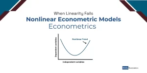
That logic also clarifies when related econometric tools should be used. If the issue is omitted-variable bias rather than stochastic trends, instrumental variables may be the relevant method. If variables are jointly determined within a system, simultaneous equations models may be needed. If the dynamics are nonlinear, nonlinear econometric models may be more suitable. Cointegration specifically addresses the validity of long-run relations among integrated time series.
MASEconomics Explains
4 economic concepts behind cointegration
These concepts are explored in depth across our educational articles library.
Explore the MASEconomics BlogConclusion
Cointegration and Engle-Granger Method give economists a disciplined way to test long-run relationships among non-stationary variables. The method begins with a levels regression, but it does not trust the levels regression by itself. It tests whether the residual is stationary. If the residual has no unit root, the variables are cointegrated, and the long-run equation has statistical meaning. If the residual has a unit root, the impressive levels regression may be another spurious relationship.
The core result is practical. Cointegration separates shared stochastic trends from accidental trend correlation. The Engle-Granger method is most useful when theory points to one long-run equilibrium equation, and the researcher needs a transparent residual-based test. Its limits are also clear: low power, sensitivity to normalisation, structural breaks, and inability to handle multiple cointegrating vectors in large systems. Used with those limits in mind, it remains one of the central tools of applied time-series econometrics.
Frequently Asked Questions
What is cointegration in simple terms?
Cointegration means two or more non-stationary variables share a stable long-run relationship. Each variable may wander over time, but a particular linear combination of them is stationary. In economic terms, the variables can drift in the short run while remaining tied by equilibrium forces in the long run.
What are the steps in the Engle-Granger method?
The Engle-Granger method has two main steps. First, estimate the long-run equation by OLS and save the residuals. Second, test those residuals for a unit root using a residual-based ADF test with cointegration-specific critical values. If the residual is stationary, the variables are cointegrated. A final error-correction model can then estimate short-run adjustment.
What is the null hypothesis of the Engle-Granger cointegration test?
The null hypothesis is no cointegration. In residual terms, the null states that the estimated equilibrium error has a unit root. Rejecting the null means the residual is stationary and the variables have a cointegrating relationship.
Why are Engle-Granger critical values different from ADF critical values?
Engle-Granger critical values differ because the residual being tested is generated from an estimated long-run regression. The prior estimation changes the distribution of the residual ADF statistic. Standard ADF critical values are therefore not valid for the cointegration test.
When should Johansen cointegration be used instead of Engle-Granger?
Johansen cointegration is usually preferred when the system contains more than two variables and there may be multiple cointegrating relationships. Engle-Granger is simpler and more transparent, but it is a single-equation method and cannot estimate the full cointegration rank of a multivariate system.
Thanks for reading! If you found this helpful, share it with friends and spread the knowledge. Happy learning with MASEconomics