Floating Exchange Rates Mundell-Fleming: Policy Under a Float

When the major economies abandoned fixed parities in the early 1970s and let their currencies float, central banks gained back something a peg had taken from them: control of their own money supply. A floating rate removes the obligation to defend a fixed price for the currency, so reserve flows no longer dictate the monetary base. The behavior of floating exchange rates Mundell-Fleming analysis predicts follows directly from that change, and it produces the exact mirror image of the fixed-rate case. Under a float with mobile capital, monetary policy becomes powerful while fiscal policy loses most of its punch.

That reversal is not arbitrary. It comes out of the same open-economy diagram developed by Robert Mundell and J. Marcus Fleming, where the goods market, the money market, and the external balance must clear together. The Mundell-Fleming model shows that the exchange-rate regime decides which variable absorbs an external imbalance. Under a float, that variable is the exchange rate itself, and tracing one monetary expansion through the diagram shows why letting the currency move changes everything.

Freedoms and Constraints Under a Float

A floating exchange rate is the absence of a commitment to any particular currency value. The central bank does not buy or sell foreign currency to hold a target, so the exchange rate is free to move to whatever level clears the foreign exchange market. The immediate consequence is that the money supply is no longer endogenous. The central bank sets it, and reserve flows do not force it up or down, because there is no peg to defend.

What adjusts instead is the exchange rate. When the balance of payments would otherwise run a deficit, the currency depreciates until the accounts balance; when it would run a surplus, the currency appreciates. The accounting is the same identity that underlies any analysis of the balance of payments, but the adjustment runs through the price of the currency rather than through reserves. A depreciation makes exports cheaper and imports dearer, which improves net exports and shifts the IS curve, the channel that does the work the money supply did under a peg.

In the diagram, this means the LM curve is now anchored by the central bank and moves only when policy moves it. The exchange rate enters through net exports, so a change in the currency shifts the IS curve. That single change in what adjusts is enough to overturn the closed-economy intuition of the IS-LM framework, where the exchange rate plays no role at all.

Monetary Expansion in the Diagram

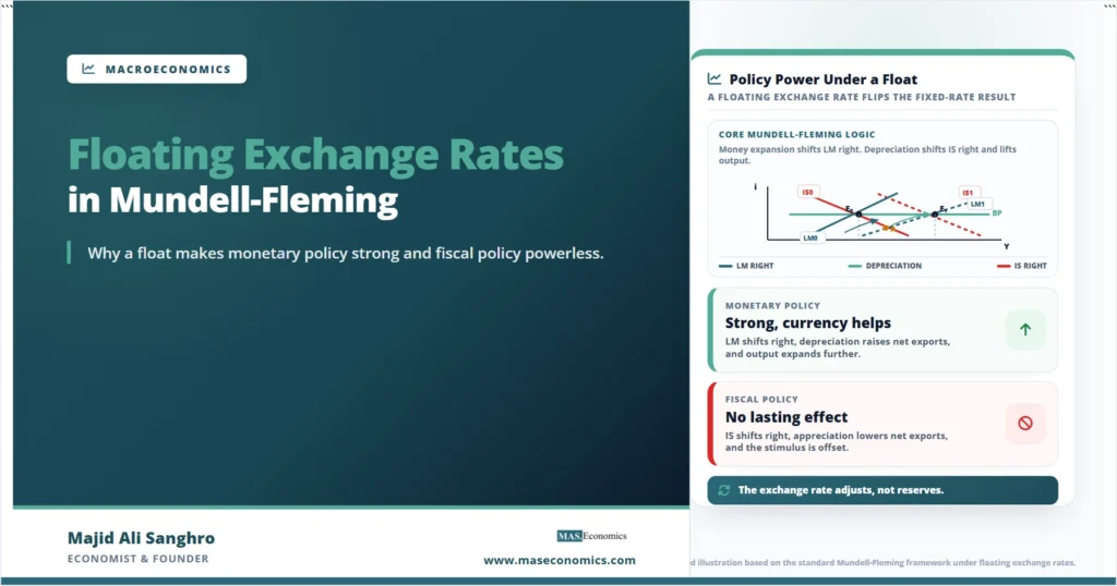
Consider a central bank that expands the money supply under a floating rate with high capital mobility, so the BP curve is relatively flat. The monetary expansion shifts the LM curve to the right. At the new internal crossing, output is higher, and the domestic interest rate is lower, which is the familiar closed-economy result.

But that crossing now sits below the BP curve. The domestic interest rate has fallen below the level consistent with external balance, and with mobile capital that gap sends capital abroad. The balance of payments moves into deficit, and under a float the currency depreciates rather than draining reserves. The depreciation makes domestic goods more competitive, net exports rise, and the IS curve shifts to the right. The adjustment continues until the economy reaches a new equilibrium back on the BP curve, at a still higher level of output.

Monetary Expansion Under Floating Exchange Rates With Capital Mobility

Stylized illustration of monetary expansion under a floating exchange rate with high capital mobility.

The path runs from E0 to the temporary point A and then to E1. Point A is where the new LM curve crosses the original IS curve, and it lies below the BP curve, the visible sign of the balance-of-payments deficit. The economy does not stay at A. The currency depreciates, net exports rise, the IS curve shifts right, and the economy settles at E1, where IS1, LM1, and BP all meet again at higher output.

The reason monetary policy is so effective here is that the exchange-rate response reinforces it. In a closed economy, the monetary expansion works only through the lower interest rate and the investment it stimulates. Under a float with mobile capital, the lower interest rate also triggers a depreciation that boosts net exports, adding a second expansionary channel on top of the first. Monetary policy gets help from the currency, and output rises by more than the closed-economy model would suggest.

Fiscal Policy Ineffectiveness Under a Float

The same exchange-rate channel that strengthens monetary policy undermines fiscal policy. Suppose the government expands spending, shifting the IS curve to the right. Output and the domestic interest rate rise at the new internal crossing, which now sits above the BP curve. With mobile capital, the higher interest rate attracts foreign funds, the balance of payments moves toward surplus, and under a float the currency appreciates.

The appreciation makes domestic goods more expensive abroad, net exports fall, and the IS curve shifts back to the left. The currency movement undoes the fiscal stimulus. Under perfect capital mobility, the offset is complete: the appreciation crowds out exactly as much net export demand as the fiscal expansion added, the IS curve returns to its starting point, and output ends up unchanged. The fiscal expansion shows up entirely as a stronger currency and a worse trade balance, not as higher output.

This is the open-economy version of crowding out. In a closed economy fiscal policy crowds out private investment through a higher interest rate. Under a float it crowds out net exports through an appreciation, and when capital is highly mobile the second effect is strong enough to neutralize fiscal policy almost entirely. The exchange rate, free to move, converts the fiscal push into a currency move rather than an output gain. The country keeps monetary autonomy, which is the trade-off described by the Mundell trilemma: a float with open capital markets buys an independent monetary policy at the cost of a stable exchange rate.

Policy Effects Side by Side

Placing the two experiments next to each other shows the reversal cleanly. The instruments are the same as under a peg; what changes is which one moves output. Under a float, the currency is the adjusting variable, and it works with monetary policy and against fiscal policy.

Table 1. Policy Effects Under a Floating Exchange Rate With High Capital Mobility

Policy action	Curve that shifts first	Exchange-rate response	Effect on output
Monetary expansion	LM shifts right	Depreciation, net exports rise	Strong increase
Monetary contraction	LM shifts left	Appreciation, net exports fall	Strong decrease
Fiscal expansion	IS shifts right	Appreciation, net exports fall	No lasting change
Fiscal contraction	IS shifts left	Depreciation, net exports rise	No lasting change
Source: MASEconomics editorial synthesis of the Mundell-Fleming floating-rate case.

The pattern is the exact reverse of the fixed-rate case, where fiscal policy is strong and monetary policy is powerless. The same diagram delivers two opposite policy worlds depending only on whether the exchange rate is fixed or floating. That symmetry is one reason the framework has lasted: a single change in the regime, with everything else held constant, swaps the roles of the two main instruments. The broader question of how the two interact when both are active is taken up in work on fiscal and monetary policy coordination.

What the Result Assumes

The sharp conclusion that fiscal policy is powerless rests on the same two assumptions that drive the fixed-rate result, applied in reverse. The first is high capital mobility, which makes the BP curve flat and the appreciation offset complete. With limited mobility, the BP curve steepens, capital responds weakly to interest-rate gaps, and fiscal policy keeps a meaningful effect on output before the currency adjustment catches up. The second is that the exchange rate moves freely and is allowed to clear the external accounts, with no managed-float intervention damping the adjustment.

A further limit is that the static diagram treats the depreciation as immediate and the price level as fixed. In practice, the exchange rate can move faster than goods prices, and the gap between the two produces dynamics the static model cannot show. The Dornbusch overshooting model was built to add exactly this, explaining why a monetary expansion can drive the currency to depreciate by more in the short run than its long-run change, before settling back. The Mundell-Fleming diagram gives the destination; the overshooting model gives the path.

Conclusion

The lesson of floating exchange rates Mundell-Fleming analysis is that letting the currency move hands monetary policy its full power and strips fiscal policy of most of its own. By freeing the exchange rate to clear the external accounts, a float lets the central bank set the money supply without fear of reserve loss, and a monetary expansion is reinforced by the depreciation it sets off. The same depreciation-and-appreciation channel that helps monetary policy turns against fiscal policy, because a fiscal expansion drives the currency up and crowds out the net exports it would otherwise have stimulated.

The driving force throughout is the free exchange rate. Under a float, the central bank chooses the money supply, and the currency, not reserves, absorbs any external imbalance. A monetary expansion that pushes the economy below the BP curve triggers a depreciation that raises net exports and lifts output further. A fiscal expansion that pushes the economy above the BP curve triggers an appreciation that lowers net exports and cancels the stimulus.

That mechanism is why the floating-rate case is the natural counterpart to the fixed-rate case rather than a separate model. Both are read off the same open-economy diagram by shifting one curve and tracing the adjustment back to external balance. Letting the exchange rate float simply assigns the adjustment to the currency, and from that single assignment the entire pattern of strong monetary policy and ineffective fiscal policy follows.

Frequently Asked Questions

Thanks for reading! If you found this helpful, share it with friends and spread the knowledge. Happy learning with MASEconomics