Quantitative Tightening Explained: What the QT Experiment Taught Us

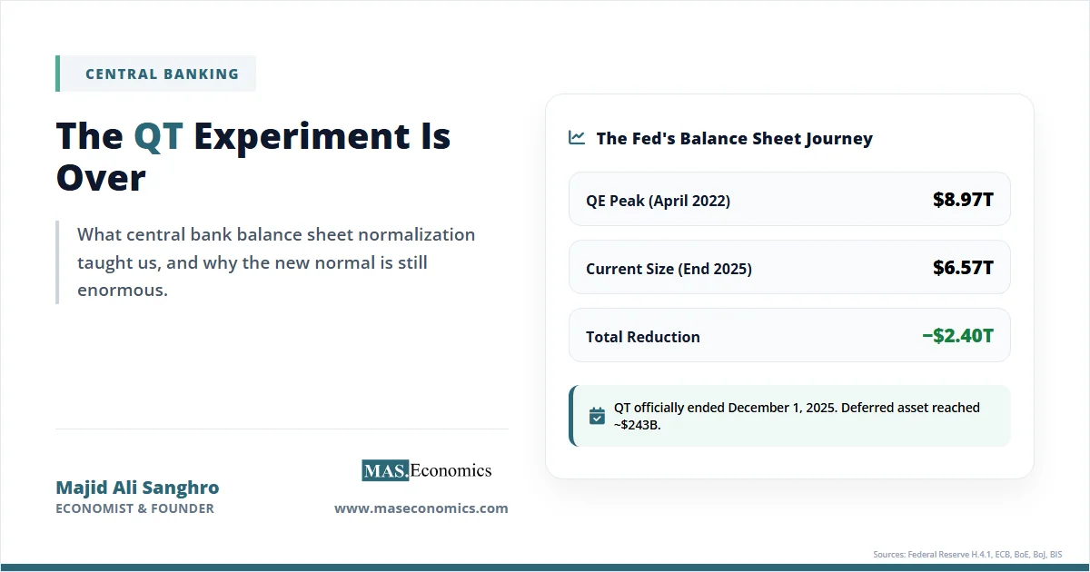
On December 1, 2025, the Federal Reserve officially ended its quantitative tightening programme, freezing its balance sheet at roughly $6.57 trillion and closing the largest attempted reversal of asset purchases in central banking history. With that single decision, the three-and-a-half-year experiment to unwind pandemic-era liquidity came to a quiet halt. The point of this article is to explain quantitative tightening as a policy tool, a set of mechanics, and above all, a stress test of modern central banking.

QT began in June 2022, when the Fed started letting Treasury and mortgage-backed securities roll off its balance sheet as part of the most aggressive anti-inflation campaign since the 1980s. The European Central Bank, Bank of England, and Bank of Japan followed, each on its own timetable and under its own constraints. By late 2025, the four major central banks had collectively withdrawn trillions of dollars of liquidity from global markets. The central question this article examines: what have we actually learned about the feasibility and the limits of balance sheet reduction?

Key Numbers Behind QT’s End

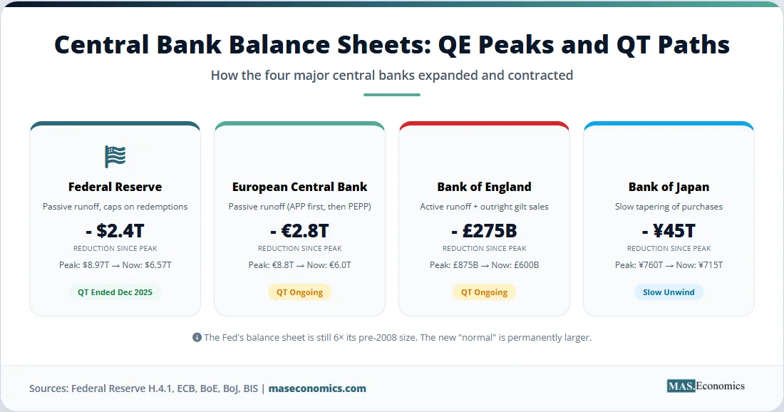
The scale of what just ended is worth stating plainly. The Fed’s balance sheet peaked near $8.97 trillion in April 2022 after two rounds of pandemic asset purchases. By the end of QT in late 2025, it had fallen to around $6.57 trillion, a reduction of roughly $2.4 trillion. Across the Fed, ECB, BoE, and BoJ, total liquidity withdrawn since mid-2022 is estimated at close to $2.4 trillion in dollar terms, a figure that would have seemed unthinkable in 2010.

Yet the endgame arrived sooner than markets expected. An earlier New York Fed survey had forecast runoff ending in the first quarter of 2026. Instead, minutes from the October 2025 FOMC meeting showed near-unanimous support for halting QT immediately on December 1, with only Governor Stephen Miran dissenting in favour of an even earlier stop. The trigger was not a dramatic blow-up. It was a quiet but persistent warning signal: the Secured Overnight Financing Rate (SOFR) had climbed above the Fed’s interest on reserves, take-up at the Standing Repo Facility had surged, and money market volatility had ticked higher through October. Reserves, at around $3.0 trillion, were not yet scarce. But policymakers had learned from 2019 that waiting for markets to break was a mistake they did not want to repeat.

What was notable about the end of QT2 was how undramatic it looked. No repo-rate spike, no emergency liquidity facilities spun up overnight, no weekend conference calls. The contrast with the first Fed runoff attempt in 2019 is the starting point of almost every honest assessment of this policy cycle.

A Timeline of QE and QT Across the Four Majors

To understand what the December 2025 decision means, the full arc of balance sheet policy across major central banks matters. The Fed’s unconventional policy began in late 2008, when the zero lower bound on interest rates forced quantitative easing onto the menu. Three rounds of QE carried the balance sheet from under $900 billion pre-crisis to roughly $4.5 trillion by 2014. A modest runoff from 2017 to 2019 shaved about $700 billion before the September 2019 repo spike forced a reversal.

The pandemic then changed the scale entirely. Between March 2020 and April 2022, the Fed nearly doubled its balance sheet again, this time buying $80 billion in Treasuries and $40 billion in mortgage-backed securities every month at the peak. The ECB’s Pandemic Emergency Purchase Programme (PEPP) took the Eurosystem balance sheet above €8.8 trillion. The BoE’s gilt purchases peaked at £875 billion. The BoJ, already the pioneer of large-scale asset purchases, ended 2022 holding more Japanese government bonds than any other entity on earth, with a balance sheet exceeding 130% of GDP.

QT arrived in staggered waves. The Fed began passive runoff in June 2022, capping monthly reductions at $47.5 billion initially, raising the cap to $95 billion by September 2022. The BoE started active QT, including outright gilt sales, in November 2022. It was the only major central bank to sell bonds rather than simply let them mature. The ECB shifted its Asset Purchase Programme (APP) portfolio to passive runoff in March 2023, then stopped reinvesting PEPP securities at the end of 2024. The BoJ moved last and least, announcing only a tapering of purchases in March 2024, before beginning to hike rates in small steps through 2025.

The figures in Table 1 pull together these four journeys on a single page.

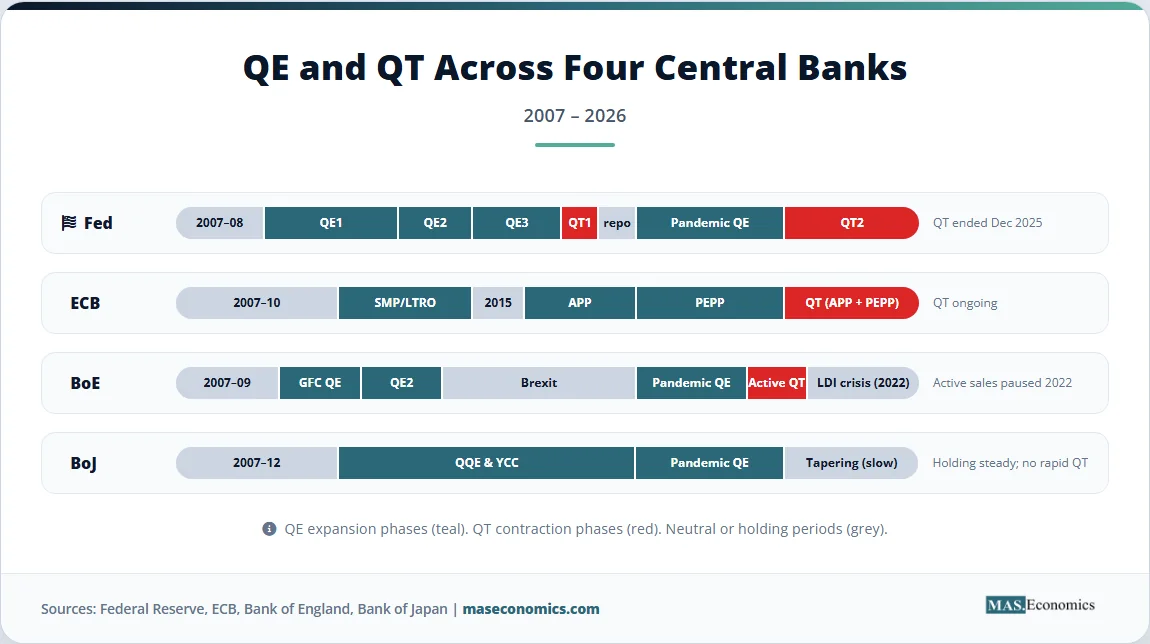
Table 1. Balance Sheet Journeys: QE Peaks and QT Paths Across Four Central Banks

Central Bank	QE Peak Size	QT Start	QT Approach	Current Size (End 2025)	Notable Feature
Federal Reserve	~$8.97 trillion (April 2022)	June 2022	Passive runoff (caps on redemptions)	~$6.57 trillion	QT officially ended December 1, 2025
European Central Bank	~€8.8 trillion (mid-2022)	March 2023	Passive runoff (APP first, then PEPP)	~€6.0 trillion	Full passive QT reached in 2025; stable money markets
Bank of England	~£875 billion (early 2022)	November 2022	Active runoff plus outright gilt sales	~£600 billion	Only major bank to actively sell; paused amid 2022 gilt crisis
Bank of Japan	~¥760 trillion (2024)	March 2024 (tapering)	Slow tapering of purchases	~¥715 trillion	Still the largest balance sheet relative to GDP

Sources: Federal Reserve H.4.1 releases; ECB weekly financial statements; Bank of England Asset Purchase Facility reports; Bank of Japan monthly balance sheet data; Bank of America Global Research QT forecasts.

The Mechanics of Balance Sheet Reduction

Most commentary treats QT as the mirror image of QE: central banks bought bonds to add liquidity, now they are letting bonds go to remove it. That is accurate at the top level but hides important details. The actual channels through which QT bites on the economy are narrower and less reliable than those of its expansionary cousin.

The core mechanic is simple. When a central bank holds a Treasury bond and that bond matures, the Treasury pays off the principal. If the central bank reinvests the proceeds in a new bond, the balance sheet stays flat. If it lets the bond mature without reinvesting, the Treasury must find that cash from the private sector instead, usually by issuing a new bond to a private buyer. The private buyer pays for the new bond by drawing down bank reserves. Bank reserves shrink. The central bank’s balance sheet shrinks by the same amount. This is “passive” QT, and it is the approach every major central bank other than the BoE has adopted.

Active QT goes further. The BoE has been selling gilts outright into the market, effectively forcing private buyers to absorb more duration risk than passive runoff alone would require. Active sales are more aggressive but also more controversial, because they can crystallise losses on securities bought at higher prices during QE.

Either way, the ultimate target is bank reserves at the central bank. Lower reserves are supposed to tighten financial conditions through three channels. First, they raise the term premium on long-dated bonds, because private investors must be compensated for holding the duration the central bank no longer wants. Second, they shrink the pool of liquid assets banks can use for market-making and repo lending, which tightens short-term funding markets. Third, they signal a contractionary stance that complements rate hikes, reinforcing the policy message. In practice, the first channel has been the weakest and the second the most dangerous.

This is where QT meets the modern “ample reserves” operating framework. Before 2008, central banks ran scarce-reserve systems in which tiny changes in reserve supply moved overnight rates sharply. After 2008, with reserves measured in trillions, central banks switched to a floor system: they pay interest on reserves at the policy rate and flood the system with liquidity, so the policy rate is set by administered rates rather than by reserve scarcity. QT works within this framework by trying to drain reserves down to the point where they are still “ample” but no longer “abundant,” close enough to the edge of scarcity to matter for balance sheet size, but not so close as to disturb money markets. Finding that point is the hardest problem in contemporary central banking.

Global Balance Sheet Trends

The chart below traces total assets of the Fed, ECB, BoE, and BoJ from 2007 through 2026. The pattern is unmistakable: three distinct QE waves (global financial crisis, eurozone sovereign debt crisis, pandemic) followed by the first serious, synchronised attempt at reversal.

Three features stand out. The first is how shallow the post-2022 reversal looks when plotted against the mountain of pandemic-era expansion. Even after the largest attempted unwind in history, each central bank’s balance sheet sits far above its 2019 level, and even further above any plausible “normal” benchmark from before 2008. The second is the divergence in approach: the Fed and ECB have both delivered meaningful reductions, the BoE has been aggressive but on a much smaller base, and the BoJ has barely moved. The third is what the chart cannot show directly: the pace of reduction has slowed markedly since mid-2024, and the Fed has now stopped entirely. The QT era, in its most active form, is over.

Three QT Warning Signs

The headline achievement of QT2 is that nothing spectacular went wrong. That framing misses the point. Things did go wrong, repeatedly and at considerable cost. The difference is that central banks had prior episodes to learn from.

The first warning came in September 2019. The Fed’s first QT attempt had reduced reserves from a peak of roughly $2.8 trillion down to about $1.4 trillion by the third quarter of that year. On September 16 and 17, the overnight repo rate, which had been trading around 2.2%, spiked to 10% intraday. The effective federal funds rate pushed above the top of the Fed’s target range, representing a temporary loss of monetary policy control. The Fed’s own subsequent analysis linked the episode to reserve scarcity interacting with month-end Treasury auction settlements and corporate tax payments. Within a week, the New York Fed was conducting emergency repo operations, and within a month, the Fed had announced it would resume Treasury bill purchases to rebuild reserves. That end of QT1 hard-coded a lesson into every central banker: the line between “ample” and “scarce” reserves is not where the models predicted it would be, and crossing it is both costly and embarrassing.

The second warning came from London in late September 2022. Following the UK government’s “mini-budget” of September 23, which announced unfunded tax cuts, thirty-year gilt yields rose by more than 100 basis points in four days. The rise triggered margin calls on liability-driven investment (LDI) funds used by UK pension schemes to hedge long-dated liabilities. To meet those margin calls, LDI funds sold gilts, driving yields higher still, triggering more margin calls, in a classic fire-sale feedback loop. Bank of England research later estimated that LDI selling accounted for roughly half the total decline in gilt prices during the crisis. The Bank was forced to intervene on September 28 with temporary gilt purchases, a balance sheet expansion in the middle of a QT programme, to restore market functioning. It paused active gilt sales for several weeks. The episode was technically a financial stability operation rather than a monetary policy reversal, but it showed how rapidly a runoff programme can collide with fragilities in the non-bank financial sector.

The third warning came from the United States in March 2023, when the collapse of Silicon Valley Bank and Signature Bank triggered broader concerns about regional bank liquidity. The Fed’s response, the Bank Term Funding Program, effectively added around $300 billion to the balance sheet in the space of weeks, temporarily reversing months of QT progress. Separately, Fed officials began talking more openly about the “lowest comfortable level of reserves,” or LCLoR, a phrase that has since become central to balance sheet debates. The LCLoR is the floor below which reserves cannot safely fall without risking money market dysfunction. The problem is that no one knows exactly where that floor is until it is breached, and the floor itself is a moving target that depends on bank regulation, Treasury issuance patterns, and the size of the reverse repo facility.

Three episodes, three different shocks, one common lesson: balance sheet reduction is not a passive technical exercise. It is a live experiment in which the demand curve for reserves is only visible after the fact.

Why Normalization Is So Hard

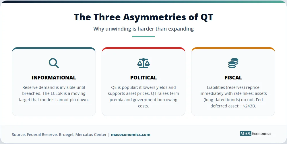
The practical difficulty of QT is not simply a calibration problem. It reflects deeper asymmetries between expansion and contraction in the modern central bank toolkit.

The first asymmetry is informational. When a central bank expands its balance sheet, it floods the system with reserves, and any excess simply sits there, earning interest. Over-supply is costless to the financial system and is quickly absorbed. But when a central bank contracts its balance sheet, it approaches a threshold below which markets break. Because reserve demand depends on bank regulation, payment system design, Treasury balances, and the size of the overnight reverse repo facility, that threshold is not observable in advance. Each central bank has tried different methods to estimate it. Fed researchers have modeled demand using the spread between the effective federal funds rate and the interest on reserves, suggesting a U.S. floor somewhere between $2.8 trillion and $3.5 trillion. The Bank of England surveyed its own counterparties directly, arriving at a range of £150 billion to £250 billion in needed reserves. The ECB has leaned on short-rate models. All of these estimates are imprecise, and all of them shift over time.

The second asymmetry is political. QE is, in political terms, almost frictionless. It lowers long-term yields, supports asset prices, and reduces government borrowing costs. Treasury officials rarely complain. QT does the opposite: it pushes up term premia, drags on risk assets, and raises the government’s effective cost of funding. This asymmetry shapes how monetary and fiscal policy interact. When central banks shrink their holdings of government debt, the private sector must absorb more, typically at higher yields. When the Treasury is simultaneously running large deficits, the combined supply of duration can overwhelm demand, as UK experience in 2022 demonstrated. QT expansion is politically popular; QT contraction is politically expensive, which is why every central bank has hesitated to push it to its theoretical limit.

The third asymmetry is fiscal. The Fed has recorded negative net income since September 2022, because the interest rate it pays on bank reserves and reverse repos now exceeds the average yield on the securities it holds. By late 2025, the cumulative deferred asset, an accounting placeholder for losses the Fed must earn back before resuming payments to the Treasury, had reached roughly $243 billion. Remittances to the Treasury, which had averaged about $100 billion per year during the QE era, fell close to zero for the first time since 1934. Mercatus Center analysis suggests remittances may not resume in normal size until 2028 or later. In fiscal terms, QT is costly precisely because the liabilities (interest on reserves) reprice immediately with rate hikes, while the assets (long-dated Treasuries and mortgage-backed securities) pay the low coupons set at the time of purchase. This is a structural by-product of the ample reserves regime, not a policy mistake, but it imposes a real fiscal cost that was invisible during QE.

QT Lessons Learned

With the Fed’s runoff now frozen and the ECB’s balance sheet still shrinking at a measured pace, it is possible to draw a preliminary ledger. Table 2 collects the main lessons from the QT2 experience across the four major central banks.

Table 2. Lessons from QT: What Worked, What Failed, and What Comes Next

Area	What Worked	What Failed or Surprised	What Is Next
Market impact	Passive runoff did not trigger a sustained rise in term premia.	Signalling channel proved weaker than expected; QT mainly mattered for short-rate markets.	Central banks will likely treat QT as a complement to rates, not a substitute.
Money markets	New standing facilities (Fed SRF, BoE STR) reduced the risk of 2019-style spikes.	SOFR drifted above IORB in autumn 2025, forcing an earlier-than-planned end to QT.	Expect permanent reserve management via T-bill purchases, not runoff.
Financial stability	BoE 2022 and SVB 2023 responses show central banks can pivot quickly when needed.	LDI crisis, regional bank stress, and repo pressures all surfaced during QT.	Tighter non-bank regulation and new liquidity tools to prevent future episodes.
Fiscal side	QT reduced the central bank’s footprint in sovereign debt markets.	Fed deferred asset rose to ~$243 billion; remittances near zero since late 2022.	Remittances unlikely to normalise before 2028; persistent fiscal cost of ample reserves.
Balance sheet size	Fed cut roughly $2.4 trillion; ECB passive QT delivered €400 billion in 2025.	Pre-2008 balance sheets are no longer a realistic benchmark.	New “steady state” around $6.5T (Fed), €5.6T (ECB by 2027); still enormous.
Cross-country comparison	BoJ avoided money market stress by moving slowly.	BoE active sales remain controversial; crystallise losses at unfavourable prices.	Divergent paths likely to continue as rate cycles diverge.

Sources: Federal Reserve communications (October 2025 FOMC minutes); Bank of England Quarterly Bulletin (2023); European Central Bank Economic Bulletin; Bank of Japan Outlook Report; BIS Quarterly Review; Bruegel Policy Brief on ECB QT.

Policy Actions and Limits

Two features of the end of QT2 deserve emphasis. Neither is a panacea, and neither resolves the underlying tension between balance sheet size and monetary discipline.

The first is technical. The Fed has indicated that once QT ends, the principal from maturing mortgage-backed securities, roughly $16 billion a month, will be reinvested into Treasury bills rather than longer-dated coupon Treasuries. This achieves two goals. It keeps the balance sheet stable in size while shortening its duration, and it adds a steady buyer at the short end of the Treasury curve, which should support money market functioning. It is not QE. It is balance sheet maintenance, equivalent to the Bank of Canada’s stated plan to “grow passively with currency demand” once its own runoff ends. Similar thinking shapes the modern central bank toolkit.

The second is political. The Fed ended QT against a political backdrop that was, candidly, uncomfortable. A substantial deferred asset, visible losses on government bond holdings, and vocal criticism from parts of the policy community about an outsized central bank footprint have all put balance sheet policy under scrutiny. This is one strand of a wider debate about central bank independence in the current transition. Ending QT on schedule was, among other things, a technical decision. It was also a signal that the Fed was prepared to adjust when markets signalled strain, rather than pushing on with a symbolic commitment to a smaller balance sheet.

On the question of whether central banks will ever return to pre-2008 balance sheets, the honest answer is: almost certainly not. Three factors lock in larger footprints. Currency in circulation has more than doubled since 2008. Bank regulation now requires far larger stocks of high-quality liquid assets, and reserves are the highest-quality of all. And the operating framework has changed: the floor system the Fed adopted in 2008 requires ample reserves by design. A return to the $900 billion balance sheet of 2007 would require reverting to a scarce-reserves system with much more volatile overnight rates, which no major central bank has signalled any intention of doing. The new “normal” is somewhere around $6.0 to $6.5 trillion for the Fed and €5.5 to €6.0 trillion for the ECB, still six to seven times their pre-crisis size.

The fiscal implications of this new steady state are already apparent and will persist. A central bank that holds trillions of long-dated assets funded by interest-bearing reserves will lose money whenever short rates are high relative to the coupons on its holdings. That drag flows directly through to the government budget via reduced remittances. Over the medium term, this will feature in debates about the interaction between central bank balance sheets and fiscal policy, and about how interest rate decisions by major central banks shape government financing costs. It will also shape the increasingly divergent paths of the major central banks in 2026, as each weighs the political cost of persistent operating losses against the financial stability benefits of ample reserves. For a broader primer on the framework within which these choices sit, the MASEconomics introduction to central banking and monetary policy provides the full context.

MASEconomics Explains

Conclusion

The QT experiment is over, at least at the Fed, and the verdict is mixed. Quantitative tightening explained is a tool that worked better than the 2019 episode suggested it could, but not as smoothly as policymakers hoped. Roughly $2.4 trillion of liquidity was withdrawn without a repeat of acute money market dysfunction, thanks in large part to new standing facilities, clearer forward guidance, and an earlier pivot than in 2019. Yet the experience also exposed the limits of balance sheet reduction: the LDI crisis, regional bank stress, rising SOFR-IORB spreads, and a persistent fiscal drag from the deferred asset all argued against pushing further. Balance sheets will remain large, remittances to governments will stay depressed, and the new normal is a permanent floor several times the size of the pre-2008 world. The deeper lesson is that QE was easier to start than to finish, and that the central bank toolkit of the next decade will be built around managing, not shrinking, the assets accumulated since 2008.

Did you find this article helpful? Share it with someone who loves economics. And remember, at MASEconomics, we make complex ideas simple.