Microeconomics often relies on visual models to unravel the complexities of resource allocation, especially when multiple agents with competing interests interact. One of the most elegant and insightful tools for analyzing exchange economies is the Edgeworth box. Named after the Irish economist Francis Ysidro Edgeworth, this diagram provides a complete picture of how two individuals can trade two goods to reach mutually beneficial outcomes.
The Edgeworth box is not just an academic exercise; it underpins fundamental concepts such as Pareto efficiency, competitive equilibrium, and the welfare theorems. By understanding this model, you gain a deeper appreciation for how markets can (and sometimes cannot) achieve efficient allocations. This article explores the Edgeworth box in detail, walking through its components, the logic of trade, and its implications for economic theory and policy.
What Is the Edgeworth Box?
The Edgeworth box is a graphical representation of a simple exchange economy with two goods and two individuals. It shows all possible allocations of the two goods between the two people, taking into account their initial endowments and preferences.
Key features of the Edgeworth box:
- Two individuals (often called A and B).
- Two goods (often labelled X and Y).
- Fixed total quantities of each good, no production, only redistribution through trade.
- Each point inside the box represents a unique allocation of the two goods between A and B.
The width of the box represents the total quantity of good X, and the height represents the total quantity of good Y. The origin for individual A is at the bottom‑left corner; the origin for individual B is at the top‑right corner, rotated 180 degrees. This clever inversion allows every possible distribution to be represented within the same rectangle.
Why two goods and two people?
The model deliberately simplifies to capture the essence of exchange. Once we understand the two‑person, two‑good case, we can generalise to many goods and many individuals conceptually, though the visual simplicity is lost.
Understanding the Edgeworth Box Diagram
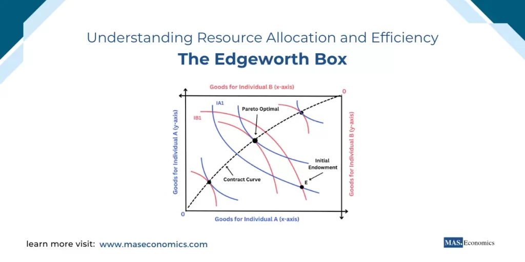
To make the model concrete, let’s examine a typical Edgeworth box diagram.
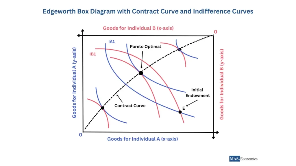
Axes and Origins
- Individual A’s goods: Measured from the bottom‑left origin. Moving right increases A’s quantity of good X; moving up increases A’s quantity of good Y.
- Individual B’s goods: Measured from the top‑right origin. Moving left increases B’s quantity of good X; moving down increases B’s quantity of good Y.
Because the total amounts of each good are fixed, any increase in A’s holdings of a good must correspond to a decrease in B’s holdings of that same good.
Initial Endowment (E)
The point labelled E marks the starting allocation of the quantities each individual initially possesses before any trade. This point reflects the initial distribution of resources, which may be unequal or inefficient.
Indifference Curves (IA₁, IB₁)
Each individual’s preferences are represented by indifference curves. For A, curves like IA₁ are drawn from the bottom‑left origin; for B, curves like IB₁ are drawn from the top‑right origin. The curves show combinations of goods that yield the same level of utility.
- Indifference curves slope downward and are convex to their respective origin (due to diminishing marginal rate of substitution).
- Higher curves (further from A’s origin) represent higher utility for A; for B, higher curves are those closer to A’s origin (since B’s utility increases as they receive more goods).
Contract Curve
The contract curve is the line (or set of points) connecting all tangency points between A’s and B’s indifference curves. Along this curve, the marginal rates of substitution of the two individuals are equal, meaning no further mutually beneficial trade is possible. All points on the contract curve are Pareto efficient.
In the diagram, the contract curve is shown as a dotted line from one corner of the box to the opposite corner. Any point on this curve represents an allocation where both individuals are as well off as possible given the other’s preferences.
Preferences, Indifference Curves, and the Marginal Rate of Substitution
To fully understand the Edgeworth box, we must delve deeper into the concept of indifference curves and the marginal rate of substitution (MRS).
Indifference Curves
An indifference curve for an individual shows all combinations of goods that yield the same level of satisfaction. Key properties:
- Downward sloping: To keep utility constant, if you get more of one good, you must give up some of the other.
- Convex to the origin: Individuals prefer balanced bundles to extreme ones (diminishing MRS).
- Higher curves = higher utility: Moving northeast for A (more of both goods) increases utility.
Marginal Rate of Substitution (MRS)
The MRS is the rate at which an individual is willing to trade one good for another while remaining equally satisfied. It is the absolute value of the slope of the indifference curve. Mathematically:
\( MRS_{XY} = \frac{MU_X}{MU_Y} \)
where \( MU_X \) and \( MU_Y \) are the marginal utilities of X and Y.
The MRS declines as we move along an indifference curve; an individual needs to give up fewer units of Y to obtain an additional unit of X when they already have a lot of X relative to Y.
Why MRS Matters in Trade
For trade to be mutually beneficial, the two individuals must have different MRS at the initial endowment. If A’s MRS is higher than B’s, it means A values X more relative to Y than B does. A would be willing to give up Y to get X, and B would be willing to give up X to get Y. They can trade until their MRS are equal, the condition for Pareto efficiency.
The Exchange Economy: Initial Endowments and Gains from Trade
The Edgeworth box models an exchange economy, a setting with no production, only redistribution of existing goods. Each individual begins with an initial endowment (point E). Because preferences differ, there may be opportunities for voluntary trade.
Why Trade Occurs
Trade happens when individuals can reallocate goods to increase their own utility without harming others. Graphically, from point E, any movement that places both individuals on a higher indifference curve (A moves to a higher IA curve, B moves to a higher IB curve) represents a mutually beneficial trade.
The set of allocations that make both individuals at least as well off as at E is called the lens formed by the intersection of the areas above A’s indifference curve through E and above B’s indifference curve through E.
All points inside this lens are potential trading outcomes.
From Initial Endowment to the Contract Curve
The trading process will continue as long as there are allocations that improve both individuals’ utility. The process stops only when the allocation reaches a point where A’s indifference curve is tangent to B’s, i.e., a point on the contract curve. At that point, no further mutually beneficial trade exists.
Key insight: The Edgeworth box shows that starting from any initial endowment, if individuals can freely trade, they will eventually reach a Pareto efficient allocation on the contract curve. The exact point they end up at depends on their bargaining power and the trading mechanism.
A Numerical Example: From Endowment to Efficiency
Let’s work through a concrete example to solidify the concepts.
Setup
- Two goods: Apples (X) and Bananas (Y).
- Total apples: 10. Total bananas: 10.
- Individual A’s initial endowment: (8 apples, 2 bananas).
- Individual B’s initial endowment: (2 apples, 8 bananas).
- Preferences: A’s utility function: \( U_A = X_A^{0.5} Y_A^{0.5} \) (Cobb‑Douglas). B’s utility function: \( U_B = X_B^{0.5} Y_B^{0.5} \).
Step 1: Compute MRS at the initial endowment
For Cobb‑Douglas, \( MRS = Y/X \) (for both individuals).
A: \( MRS_A = 2/8 = 0.25 \)
B: \( MRS_B = 8/2 = 4 \)
Since MRS differ, trade is possible. A values bananas more relative to apples than B does (A’s MRS is low, meaning A would give up many apples for one banana; B’s MRS is high, meaning B would give up many bananas for one apple).
Step 2: Find the contract curve
For these Cobb‑Douglas preferences, the contract curve is the set of allocations where \( Y_A / X_A = Y_B / X_B \) (since MRS equality implies equal ratios). Using the total constraints \( X_B = 10 – X_A \), \( Y_B = 10 – Y_A \), we get:
Solving yields \( Y_A = X_A \). So the contract curve is the diagonal from (0,0) to (10,10) in A’s coordinates.
Step 3: Find a Pareto efficient allocation reachable from the endowment
Suppose A and B trade until A ends up with (5 apples, 5 bananas) and B with (5 apples, 5 bananas). Then both have the same ratio, MRS = 1 for both. This point lies on the contract curve. Both are better off than at the endowment (utility increases from \( \sqrt{8 \times 2} = 4 \) to \( \sqrt{5 \times 5} = 5 \) for A, similarly for B).
This simple example illustrates how trade moves the economy to an efficient outcome.
Pareto Efficiency and the Contract Curve
An allocation is Pareto efficient (or Pareto optimal) if there is no alternative allocation that makes at least one individual better off without making the other worse off.
In the Edgeworth box, the contract curve is the set of all Pareto efficient allocations. It consists of points where the indifference curves of the two individuals are tangent, meaning their marginal rates of substitution are equal.
Properties of the Contract Curve
- Equality of MRS: At any point on the contract curve, \( MRS_A = MRS_B \).
- No waste: All goods are fully allocated; nothing is left unused.
- Optimality: Any movement away from the contract curve would make at least one person worse off.
The contract curve runs from the bottom‑left corner to the top‑right corner, but its shape depends on the specific preferences of the two individuals.
Competitive Equilibrium in the Edgeworth Box
The Edgeworth box is also used to illustrate the concept of competitive equilibrium. In a competitive market, individuals take prices as given and choose the best affordable bundle.
How Competitive Equilibrium Works
- Prices (relative price of good X in terms of good Y) are announced.
- Each individual has an initial endowment, which gives them a budget line (or budget constraint) based on those prices.
- Individuals maximise utility subject to their budget.
- Market clearing requires that the total demand for each good equals the total supply (the fixed quantities in the box).
In the diagram, a competitive equilibrium occurs at a point where:
- For each individual, the budget line is tangent to their indifference curve.
- The two budget lines coincide (since there is only one price ratio).
- The resulting allocation lies on the contract curve.
Thus, competitive equilibrium allocations are always Pareto efficient, a result known as the First Welfare Theorem.
The First and Second Welfare Theorems
The Edgeworth box provides an intuitive foundation for two fundamental theorems of welfare economics.
First Welfare Theorem
If markets are competitive and complete, and there are no externalities or market failures, then any competitive equilibrium is Pareto efficient. In the Edgeworth box, this means that the equilibrium point (where budget lines are tangent to indifference curves) always lies on the contract curve.
Intuition: In a competitive market, if there were an inefficiency (a point not on the contract curve), someone could propose a trade that makes both better off. That trade would be a profitable opportunity, contradicting the equilibrium.
Second Welfare Theorem
Conversely, any Pareto efficient allocation can be achieved as a competitive equilibrium by appropriately redistributing initial endowments. In other words, society can choose a desirable, efficient outcome (e.g., a fairer distribution) and then let markets work to reach it, provided initial endowments are adjusted accordingly.
Intuition: Given any point on the contract curve, we can find a budget line that is tangent to both indifference curves at that point. If we redistribute endowments so that the budget line passes through the new endowment point, the market will lead to that efficient allocation.
These theorems form the theoretical basis for the belief that markets can be efficient, but also highlight the importance of initial distribution, a point often debated in policy discussions.
Extending to More Than Two Individuals
When there are more than two individuals, the Edgeworth box (two dimensions) cannot capture all interactions. However, the concept extends to the core of an economy.
The core is the set of allocations that no coalition can improve upon. In a two‑person economy, the core is exactly the contract curve (provided there are no other constraints). With many individuals, the core is a subset of the set of Pareto efficient allocations, shrinking as the number of agents grows. In perfectly competitive markets (with many agents), the core converges to the set of competitive equilibria, a result known as the limit theorem of the core.
This convergence shows that the Edgeworth box intuition scales up: competitive markets lead to efficient outcomes even with many participants.
Production and the Edgeworth Box
The Edgeworth box can be extended to include production by combining it with a production possibility frontier. This gives the Edgeworth box in production or the production‑exchange economy.
In such a model, we have:
- Two goods (X and Y) and two factors (labour and capital).
- An Edgeworth box in factor space shows efficient input allocations.
- A production possibility frontier derived from that box shows the trade‑off in output.
- A second Edgeworth box (or a separate diagram) shows exchange between consumers given the outputs.
The combined model demonstrates the fundamental theorems of welfare economics in a full general equilibrium setting. This framework also forms the basis for modern international trade theories, such as the Heckscher‑Ohlin model and the Rybczynski theorem, which examine how factor endowments and growth affect trade patterns.
Limitations of the Edgeworth Box
While the Edgeworth box is a powerful teaching tool, it has limitations:
- Only two goods and two individuals in real economies have many goods and agents.
- No production models, pure exchange, not production economies.
- Assumes perfect divisibility, goods can be split arbitrarily.
- No transaction costs or information asymmetries.
- Assumes fixed total quantities, no growth or innovation.
Despite these simplifications, the insights about gains from trade, efficiency, and competitive equilibrium remain central to modern microeconomics.
Conclusion
The Edgeworth box is more than a diagram; it is a concise representation of the logic of exchange, the gains from trade, and the conditions for market efficiency. By mapping initial endowments, preferences, and trading possibilities onto a single graph, it shows how voluntary trade can move an economy from an arbitrary starting point to a Pareto efficient outcome.
Whether you are studying microeconomics, analysing international trade, or simply trying to understand how markets work, the Edgeworth box provides an indispensable visual foundation. Its lessons that trade benefits all parties when preferences differ, and that competitive markets lead to efficient allocations, remain cornerstones of economic thought.
FAQs:
What is the Edgeworth box?
The Edgeworth box is a graphical tool used in microeconomics to analyze how two individuals allocate two goods between themselves, considering their preferences and initial endowments. It highlights the conditions for mutually beneficial trade and efficient outcomes.
What does the initial endowment represent?
The initial endowment is the starting allocation of goods each individual possesses before any trading occurs. It serves as the baseline point for analysis in the Edgeworth box.
What are indifference curves in the Edgeworth box?
Indifference curves represent combinations of goods that provide the same level of utility to an individual. These curves help visualize preferences and the trade-offs individuals are willing to make.
What is Pareto efficiency in the context of the Edgeworth box?
An allocation is Pareto efficient if no individual can be made better off without making the other worse off. The contract curve within the Edgeworth box connects all Pareto efficient allocations.
What is the contract curve?
The contract curve is the set of all Pareto efficient allocations where both individuals maximize their utility, and no further mutually beneficial trades are possible.
How does trade occur in the Edgeworth box?
Trade occurs when individuals move from their initial endowment toward a point on the contract curve. These trades are voluntary and improve both individuals’ utilities until no further gains are possible.
What is a competitive equilibrium in the Edgeworth box?
A competitive equilibrium occurs when both individuals maximize their utility given market prices, and the allocation is Pareto efficient. At this point, the indifference curves of both individuals are tangent, reflecting no further gains from trade.
Why is the Edgeworth box important?
The Edgeworth box provides insights into resource allocation, trade, and efficiency. It demonstrates how individuals can achieve mutually beneficial outcomes and helps explain the conditions for market efficiency in an exchange economy.
Thanks for reading! Share this with friends and spread the knowledge if you found it helpful.
Happy learning with MASEconomics